Compliance Just Got Easier: Stay ahead of regulatory changes with instant notifications on updates that matter.
['Oil Spill Prevention', 'CERCLA, SARA, EPCRA']
['Oil Spills', 'SARA Compliance', 'Contingency Planning', 'Superfund', 'CERCLA, SARA, EPCRA', 'Toxic/Hazardous Substance Releases']
12/22/2025

Copyright 2026 J. J. Keller & Associate, Inc. For re-use options please contact copyright@jjkeller.com or call 800-558-5011.
Table of Contents
List of Figures
List of Tables
1.0. Introduction.
1.1 Definitions.
2.0 Evaluations Common to Multiple Pathways.
2.1 Overview.
2.1.1 Calculation of HRS site score.
2.1.2 Calculation of pathway score.
2.1.3 Common evaluations.
2.2 Characterize sources.
2.2.1 Identify sources.
2.2.2 Identify hazardous substances associated with a source.
2.2.3 Identify hazardous substances available to a pathway.
2.3 Likelihood of release.
2.4 Waste characteristics.
2.4.1 Selection of substance potentially posing greatest hazard.
2.4.1.1 Toxicity factor.
2.4.1.2 Hazardous substance selection.
2.4.2 Hazardous waste quantity.
2.4.2.1 Source hazardous waste quantity.
2.4.2.1.1 Hazardous constituent quantity.
2.4.2.1.2 Hazardous wastestream quantity.
2.4.2.1.3 Volume.
2.4.2.1.4 Area.
2.4.2.1.5 Calculation of source hazardous waste quantity value.
2.4.2.2 Calculation of hazardous waste quantity factor value.
2.4.3 Waste characteristics factor category value.
2.4.3.1 Factor category value.
2.4.3.2 Factor category value, considering bioaccumulation potential.
2.5 Targets.
2.5.1 Determination of level of actual contamination at a sampling location.
2.5.2 Comparison to benchmarks.
3.0 Ground Water Migration Pathway.
3.0.1 General considerations.
3.0.1.1 Ground water target distance limit.
3.0.1.2 Aquifer boundaries.
3.0.1.2.1 Aquifer interconnections.
3.0.1.2.2 Aquifer discontinuities.
3.0.1.3 Karst aquifer.
3.1 Likelihood of release.
3.1.1 Observed release.
3.1.2 Potential to release.
3.1.2.1 Containment.
3.1.2.2 Net precipitation.
3.1.2.3 Depth to aquifer.
3.1.2.4 Travel time.
3.1.2.5 Calculation of potential to release factor value.
3.1.3 Calculation of likelihood of release factor category value.
3.2 Waste characteristics.
3.2.1 Toxicity/mobility.
3.2.1.1 Toxicity.
3.2.1.2 Mobility.
3.2.1.3 Calculation of toxicity/mobility factor value.
3.2.2 Hazardous waste quantity.
3.2.3 Calculation of waste characteristics factor category value.
3.3 Targets.
3.3.1 Nearest well.
3.3.2 Population.
3.3.2.1 Level of contamination.
3.3.2.2 Level I concentrations.
3.3.2.3 Level II concentrations.
3.3.2.4 Potential contamination.
3.3.2.5 Calculation of population factor value.
3.3.3 Resources.
3.3.4 Wellhead Protection Area.
3.3.5 Calculation of targets factor category value.
3.4 Ground water migration score for an aquifer.
3.5 Calculation of ground water migration pathway score.
4.0 Surface Water Migration Pathway.
4.0.1 Migration components.
4.0.2 Surface water categories.
4.1 Overland/flood migration component.
4.1.1 General considerations.
4.1.1.1 Definition of hazardous substance migration path for overland/flood migration component.
4.1.1.2 Target distance limit.
4.1.1.3 Evaluation of overland/flood migration component.
4.1.2 Drinking water threat.
4.1.2.1 Drinking water threat-likelihood of release.
4.1.2.1.1 Observed release.
4.1.2.1.2 Potential to release.
4.1.2.1.2.1 Potential to release by overland flow.
4.1.2.1.2.1.1 Containment.
4.1.2.1.2.1.2 Runoff.
4.1.2.1.2.1.3 Distance to surface water.
4.1.2.1.2.1.4 Calculation of factor value for potential to release by overland flow.
4.1.2.1.2.2 Potential to release by flood.
4.1.2.1.2.2.1 Containment (flood).
4.1.2.1.2.2.2 Flood frequency.
4.1.2.1.2.2.3 Calculation of factor value for potential to release by flood.
4.1.2.1.2.3 Calculation of potential to release factor value.
4.1.2.1.3 Calculation of drinking water threat-likelihood of release factor category value.
4.1.2.2 Drinking water threat-waste characteristics.
4.1.2.2.1 Toxicity/persistence.
4.1.2.2.1.1 Toxicity.
4.1.2.2.1.2 Persistence.
4.1.2.2.1.3 Calculation of toxicity/persistence factor value.
4.1.2.2.2 Hazardous waste quantity.
4.1.2.2.3 Calculation of drinking water threat-waste characteristics factor category value.
4.1.2.3 Drinking water threat-targets.
4.1.2.3.1 Nearest intake.
4.1.2.3.2 Population.
4.1.2.3.2.1 Level of contamination.
4.1.2.3.2.2 Level I concentrations.
4.1.2.3.2.3 Level II concentrations.
4.1.2.3.2.4 Potential contamination.
4.1.2.3.2.5 Calculation of population factor value.
4.1.2.3.3 Resources.
4.1.2.3.4 Calculation of drinking water threat-targets factor category value.
4.1.2.4 Calculation of the drinking water threat score for a watershed.
4.1.3 Human food chain threat.
4.1.3.1 Human food chain threat-likelihood of release.
4.1.3.2 Human food chain threat-waste characteristics.
4.1.3.2.1 Toxicity/persistence/bioaccumulation.
4.1.3.2.1.1 Toxicity.
4.1.3.2.1.2 Persistence.
4.1.3.2.1.3 Bioaccumulation potential.
4.1.3.2.1.4 Calculation of toxicity/persistence/bioaccumulation factor value.
4.1.3.2.2 Hazardous waste quantity.
4.1.3.2.3 Calculation of human food chain threat-waste characteristics factor category value.
4.1.3.3 Human food chain threat-targets.
4.1.3.3.1 Food chain individual.
4.1.3.3.2 Population.
4.1.3.3.2.1 Level I concentrations.
4.1.3.3.2.2 Level II concentrations.
4.1.3.3.2.3 Potential human food chain contamination.
4.1.3.3.2.4 Calculation of population factor value.
4.1.3.3.3 Calculation of human food chain threat-targets factor category value.
4.1.3.4 Calculation of human food chain threat score for a watershed.
4.1.4 Environmental threat.
4.1.4.1 Environmental threat-likelihood of release.
4.1.4.2 Environmental threat-waste characteristics.
4.1.4.2.1 Ecosystem toxicity/persistence/bioaccumulation.
4.1.4.2.1.1 Ecosystem toxicity.
4.1.4.2.1.2 Persistence.
4.1.4.2.1.3 Ecosystem bioaccumulation potential.
4.1.4.2.1.4 Calculation of ecosystem toxicity/persistence/bioaccumulation factor value.
4.1.4.2.2 Hazardous waste quantity.
4.1.4.2.3 Calculation of environmental threat-waste characteristics factor category value.
4.1.4.3 Environmental threat-targets.
4.1.4.3.1 Sensitive environments.
4.1.4.3.1.1 Level I concentrations.
4.1.4.3.1.2 Level II concentrations.
4.1.4.3.1.3 Potential contamination.
4.1.4.3.1.4 Calculation of environmental threat-targets factor category value.
4.1.4.4 Calculation of environmental threat score for a watershed.
4.1.5 Calculation of overland/flood migration component score for a watershed.
4.1.6 Calculation of overland/flood migration component score.
4.2 Ground water to surface water migration component.
4.2.1 General Considerations.
4.2.1.1 Eligible surface waters.
4.2.1.2 Definition of hazardous substance migration path for ground water to surface water migration component.
4.2.1.3 Observed release of a specific hazardous substance to surface water in-water segment.
4.2.1.4 Target distance limit.
4.2.1.5 Evaluation of ground water to surface water migration component.
4.2.2 Drinking water threat.
4.2.2.1 Drinking water threat-likelihood of release.
4.2.2.1.1 Observed release.
4.2.2.1.2 Potential to release.
4.2.2.1.3 Calculation of drinking water threat-likelihood of release factor category value.
4.2.2.2 Drinking water threat-waste characteristics.
4.2.2.2.1 Toxicity/mobility/persistence.
4.2.2.2.1.1 Toxicity.
4.2.2.2.1.2 Mobility.
4.2.2.2.1.3 Persistence.
4.2.2.2.1.4 Calculation of toxicity/mobility/persistence factor value.
4.2.2.2.2 Hazardous waste quantity.
4.2.2.2.3 Calculation of drinking water threat-waste characteristics factor category value.
4.2.2.3 Drinking water threat-targets.
4.2.2.3.1 Nearest intake.
4.2.2.3.2 Population.
4.2.2.3.2.1 Level I concentrations.
4.2.2.3.2.2 Level II concentrations.
4.2.2.3.2.3 Potential contamination.
4.2.2.3.2.4 Calculation of population factor value.
4.2.2.3.3 Resources.
4.2.2.3.4 Calculation of drinking water threat-targets factor category value.
4.2.2.4 Calculation of drinking water threat score for a watershed.
4.2.3 Human food chain threat.
4.2.3.1 Human food chain threat-likelihood of release.
4.2.3.2 Human food chain threat-waste characteristics.
4.2.3.2.1 Toxicity/mobility/persistence/bioaccumulation.
4.2.3.2.1.1 Toxicity.
4.2.3.2.1.2 Mobility.
4.2.3.2.1.3 Persistence.
4.2.3.2.1.4 Bioaccumulation potential.
4.2.3.2.1.5 Calculation of toxicity/mobility/persistence/bioaccumulation factor value.
4.2.3.2.2 Hazardous waste quantity.
4.2.3.2.3 Calculation of human food chain threat-waste characteristics factor category value.
4.2.3.3 Human food chain threat-targets.
4.2.3.3.1 Food chain individual.
4.2.3.3.2 Population.
4.2.3.3.2.1 Level I concentrations.
4.2.3.3.2.2 Level II concentrations.
4.2.3.3.2.3 Potential human food chain contamination.
4.2.3.3.2.4 Calculation of population factor value.
4.2.3.3.3 Calculation of human food chain threat-targets factor category value.
4.2.3.4 Calculation of human food chain threat score for a watershed.
4.2.4 Environmental threat.
4.2.4.1 Environmental threat-likelihood of release.
4.2.4.2 Environmental threat-waste characteristics.
4.2.4.2.1 Ecosystem toxicity/mobility/persistence/bioaccumulation.
4.2.4.2.1.1 Ecosystem toxicity.
4.2.4.2.1.2 Mobility.
4.2.4.2.1.3 Persistence.
4.2.4.2.1.4 Ecosystem bioaccumulation potential.
4.2.4.2.1.5 Calculation of ecosystem toxicity/mobility/persistence/bioaccumulation factor value.
4.2.4.2.2 Hazardous waste quantity.
4.2.4.2.3 Calculation of environmental threat-waste characteristics factor category value.
4.2.4.3 Environmental threat-targets.
4.2.4.3.1 Sensitive environments.
4.2.4.3.1.1 Level I concentrations.
4.2.4.3.1.2 Level II concentrations.
4.2.4.3.1.3 Potential contamination.
4.2.4.3.1.4 Calculation of environmental threat-targets factor category value.
4.2.4.4 Calculation of environmental threat score for a watershed.
4.2.5 Calculation of ground water to surface water migration component score for a watershed.
4.2.6 Calculation of ground water to surface water migration component score.
4.3 Calculation of surface water migration pathway score.
5.0 Soil Exposure and Subsurface Intrusion Pathway.
5.0.1 Exposure components.
5.1 Soil exposure component.
5.1.0 General considerations.
5.1.1 Resident population threat.
5.1.1.1 Likelihood of exposure.
5.1.1.2 Waste characteristics.
5.1.1.2.1 Toxicity.
5.1.1.2.2 Hazardous waste quantity.
5.1.1.2.3 Calculation of waste characteristics factor category value.
5.1.1.3 Targets.
5.1.1.3.1 Resident individual.
5.1.1.3.2 Resident population.
5.1.1.3.2.1 Level I concentrations.
5.1.1.3.2.2 Level II concentrations.
5.1.1.3.2.3 Calculation of resident population factor value.
5.1.1.3.3 Workers.
5.1.1.3.4 Resources.
5.1.1.3.5 Terrestrial sensitive environments.
5.1.1.3.6 Calculation of resident population targets factor category value.
5.1.1.4 Calculation of resident population threat score.
5.1.2 Nearby population threat.
5.1.2.1 Likelihood of exposure.
5.1.2.1.1 Attractiveness/accessibility.
5.1.2.1.2 Area of contamination.
5.1.2.1.3 Likelihood of exposure factor category value.
5.1.2.2 Waste characteristics.
5.1.2.2.1 Toxicity.
5.1.2.2.2 Hazardous waste quantity.
5.1.2.2.3 Calculation of waste characteristics factor category value.
5.1.2.3 Targets.
5.1.2.3.1 Nearby individual.
5.1.2.3.2 Population within 1 mile.
5.1.2.3.3 Calculation of nearby population targets factor category value.
5.1.2.4 Calculation of nearby population threat score.
5.1.3 Calculation of soil exposure component score.
5.2 Subsurface intrusion component.
5.2.0 General considerations.
5.2.1 Subsurface intrusion component.
5.2.1.1 Likelihood of exposure.
5.2.1.1.1 Observed exposure.
5.2.1.1.2 Potential for exposure.
5.2.1.1.2.1 Structure containment.
5.2.1.1.2.2 Depth to contamination.
5.2.1.1.2.3 Vertical migration.
5.2.1.1.2.4 Vapor migration potential.
5.2.1.1.2.5 Calculation of potential for exposure factor value.
5.2.1.1.3 Calculation of likelihood of exposure factor category value.
5.2.1.2 Waste characteristics.
5.2.1.2.1 Toxicity/degradation.
5.2.1.2.1.1 Toxicity.
5.2.1.2.1.2 Degradation.
5.2.1.2.1.3 Calculation of toxicity/degradation factor value.
5.2.1.2.2 Hazardous waste quantity.
5.2.1.2.3 Calculation of waste characteristics factor category value.
5.2.1.3 Targets.
5.2.1.3.1 Exposed individual.
5.2.1.3.2 Population.
5.2.1.3.2.1 Level I concentrations.
5.2.1.3.2.2 Level II concentrations.
5.2.1.3.2.3 Population within area(s) of subsurface contamination.
5.2.1.3.2.4 Calculation of population factor value.
5.2.1.3.3 Resources.
5.2.1.3.4 Calculation of targets factor category value.
5.2.2 Calculation of subsurface intrusion component score.
5.3 Calculation of the soil exposure and subsurface intrusion pathway score.
5.3 Calculation of soil exposure pathway score.
6.0 Air Migration Pathway.
6.1 Likelihood of release.
6.1.1 Observed release.
6.1.2 Potential to release.
6.1.2.1 Gas potential to release.
6.1.2.1.1 Gas containment.
6.1.2.1.2 Gas source type.
6.1.2.1.3 Gas migration potential.
6.1.2.1.4 Calculation of gas potential to release value.
6.1.2.2 Particulate potential to release.
6.1.2.2.1 Particulate containment.
6.1.2.2.2 Particulate source type.
6.1.2.2.3 Particulate migration potential.
6.1.2.2.4 Calculation of particulate potential to release value.
6.1.2.3 Calculation of potential to release factor value for the site.
6.1.3 Calculation of likelihood of release factor category value.
6.2 Waste characteristics.
6.2.1 Toxicity/mobility.
6.2.1.1 Toxicity.
6.2.1.2 Mobility.
6.2.1.3 Calculation of toxicity/mobility factor value.
6.2.2 Hazardous waste quantity.
6.2.3 Calculation of waste characteristics factor category value.
6.3 Targets.
6.3.1 Nearest individual.
6.3.2 Population.
6.3.2.1 Level of contamination.
6.3.2.2 Level I concentrations.
6.3.2.3 Level II concentrations.
6.3.2.4 Potential contamination.
6.3.2.5 Calculation of population factor value.
6.3.3 Resources.
6.3.4 Sensitive environments.
6.3.4.1 Actual contamination.
6.3.4.2 Potential contamination.
6.3.4.3 Calculation of sensitive environments factor value.
6.3.5 Calculation of targets factor category value.
6.4 Calculation of air migration pathway score.
7.0 Sites Containing Radioactive Substances.
7.1 Likelihood of release/likelihood of exposure.
7.1.1 Observed release/observed contamination/observed exposure.
7.1.2 Potential to release/potential for exposure.
7.2 Waste characteristics.
7.2.1 Human toxicity.
7.2.2 Ecosystem toxicity.
7.2.3 Persistence/degradation.
7.2.4 Selection of substance potentially posing greatest hazard.
7.2.5 Hazardous waste quantity.
7.2.5.1 Source hazardous waste quantity for radionuclides.
7.2.5.1.1 Radionuclide constituent quantity (Tier A).
7.2.5.1.2 Radionuclide wastestream quantity (Tier B).
7.2.5.1.3 Calculation of source hazardous waste quantity value for radionuclides.
7.2.5.2 Calculation of hazardous waste quantity factor value for radionuclides.
7.2.5.3 Calculation of hazardous waste quantity factor value for sites containing mixed radioactive and other hazardous substances.
7.3 Targets.
7.3.1 Level of contamination at a sampling location.
7.3.2 Comparison to benchmarks.
7.3.3 Weighting of targets within an area of subsurface contamination.
LIST OF FIGURES
Figure number
3-1 Overview of ground water migration pathway.
3-2 Net precipitation factor values.
4-1 Overview of surface water overland/flood migration component.
4-2 Overview of ground water to surface water migration component.
4-3 Sample determination of ground water to surface water angle.
5-1 Overview of the soil exposure and subsurface intrusion pathway.
6-1 Overview of air migration pathway.
6-2 Particulate migration potential factor values.
6-3 Particulate mobility factor values.
LIST OF TABLES
Table number
2-1 Sample pathway scoresheet.
2-2 Sample source characterization worksheet.
2-3 Observed release criteria for chemical analysis.
2-4 Toxicity factor evaluation.
2-5 Hazardous waste quantity evaluation equations.
2-6 Hazardous waste quantity factor values.
2-7 Waste characteristics factor category values.
3-1 Ground water migration pathway scoresheet.
3-2 Containment factor values for ground water migration pathway.
3-3 Monthly latitude adjusting values.
3-4 Net precipitation factor values.
3-5 Depth to aquifer factor values.
3-6 Hydraulic conductivity of geologic materials.
3-7 Travel time factor values.
3-8 Ground water mobility factor values.
3-9 Toxicity/mobility factor values.
3-10 Health-based benchmarks for hazardous substances in drinking water.
3-11 Nearest well factor values.
3-12 Distance-weighted population values for potential contamination factor for ground water migration pathway.
4-1 Surface water overland/flood migration component scoresheet.
4-2 Containment factor values for surface water migration pathway.
4-3 Drainage area values.
4-4 Soil group designations.
4-5 Rainfall/runoff values.
4-6 Runoff factor values.
4-7 Distance to surface water factor values.
4-8 Containment (flood) factor values.
4-9 Flood frequency factor values.
4-10 Persistence factor values—half-life.
4-11 Persistence factor values—log K ow
4-12 Toxicity/persistence factor values.
4-13 Surface water dilution weights.
4-14 Dilution-weighted population values for potential contamination factor for surface water migration pathway.
4-15 Bioaccumulation potential factor values.
4-16 Toxicity/persistence/bioaccumulation factor values.
4-17 Health-based benchmarks for hazardous substances in human food chain.
4-18 Human food chain population values.
4-19 Ecosystem toxicity factor values.
4-20 Ecosystem toxicity/persistence factor values.
4-21 Ecosystem toxicity/persistence/bioaccumulation factor values.
4-22 Ecological-based benchmarks for hazardous substances in surface water.
4-23 Sensitive environments rating values.
4-24 Wetlands rating values for surface water migration pathway.
4-25 Ground water to surface water migration component scoresheet.
4-26 Toxicity/mobility/persistence factor values.
4-27 Dilution weight adjustments.
4-28 Toxicity/mobility/persistence/bioaccumulation factor values.
4-29 Ecosystem toxicity/mobility/persistence factor values.
4-30 Ecosystem toxicity/mobility/persistence/bioaccumulation factor values.
5-1 Soil exposure component scoresheet.
5-2 Hazardous waste quantity evaluation equations for soil exposure component.
5-3 Health-based benchmarks for hazardous substances in soils.
5-4 Factor values for workers.
5-5 Terrestrial sensitive environments rating values.
5-6 Attractiveness/accessibility values.
5-7 Area of contamination factor values.
5-8 Nearby population likelihood of exposure factor values.
5-9 Nearby individual factor values.
5-10 Distance-weighted population values for nearby population threat.
5-11 Subsurface intrusion component scoresheet.
5-12 Structure containment.
5-13 Depth to contamination.
5-14 Effective porosity/permeability of geological materials.
5-15 Vertical migration factor values.
5-16 Values for vapor pressure and Henry's constant.
5-17 Vapor migration potential factor values for a hazardous substance.
5-18 Degradation factor value table.
5-19 Hazardous waste quantity evaluation equations for subsurface intrusion component.
5-20 Health-based benchmarks for hazardous substances in the subsurface intrusion component.
5-21 Weighting factor values for populations within an area of subsurface contamination.
6-1 Air migration pathway scoresheet.
6-2 Gas potential to release evaluation.
6-3 Gas containment factor values.
6-4 Source type factor values.
6-5 Values for vapor pressure and Henry's constant.
6-6 Gas migration potential values for a hazardous substance.
6-7 Gas migration potential values for the source.
6-8 Particulate potential to release evaluation.
6-9 Particulate containment factor values.
6-10 Particulate migration potential values.
6-11 Gas mobility factor values.
6-12 Particulate mobility factor values.
6-13 Toxicity/mobility factor values.
6-14 Health-based benchmarks for hazardous substances in air.
6-15 Air migration pathway distance weights.
6-16 Nearest individual factor values.
6-17 Distance-weighted population values for potential contamination factor for air pathway.
6-18 Wetlands rating values for air migration pathway.
7-1 HRS factors evaluated differently for radionuclides.
7-2 Toxicity factor values for radionuclides.
1.0 Introduction
The Hazard Ranking System (HRS) is the principal mechanism the U.S. Environmental Protection Agency (EPA) uses to place sites on the National Priorities List (NPL). The HRS serves as a screening device to evaluate the potential for releases of uncontrolled hazardous substances to cause human health or environmental damage. The HRS provides a measure of relative rather than absolute risk. It is designed so that it can be consistently applied to a wide variety of sites.
1.1 Definitions
Acute toxicity: Measure of toxicological responses that result from a single exposure to a substance or from multiple exposures within a short period of time (typically several days or less). Specific measures of acute toxicity used within the HRS include lethal dose 50 (LD50) and lethal concentration 50 (LC50), typically measured within a 24-hour to 96-hour period.
Ambient Aquatic Life Advisory Concentrations (AALACs): EPA's advisory concentration limit for acute or chronic toxicity to aquatic organisms as established under section 304(a)(1) of the Clean Water Act, as amended.
Ambient Water Quality Criteria (AWQC)/National Recommended Water Quality Criteria: EPA's maximum acute (Criteria Maximum Concentration or CMC) or chronic (Criterion Continuous Concentration or CCC) toxicity concentrations for protection of aquatic life and its uses as established under section 304(a)(1) of the Clean Water Act, as amended.
Bioconcentration factor (BCF): Measure of the tendency for a substance to accumulate in the tissue of an aquatic organism. BCF is determined by the extent of partitioning of a substance, at equilibrium, between the tissue of an aquatic organism and water. As the ratio of concentration of a substance in the organism divided by the concentration in water, higher BCF values reflect a tendency for substances to accumulate in the tissue of aquatic organisms. [unitless].
Biodegradation: Chemical reaction of a substance induced by enzymatic activity of microorganisms.
CERCLA: Comprehensive Environmental Response, Compensation, and Liability Act of 1980, as amended (Pub. L. 96-510, as amended).
Channelized flow: Natural geological or manmade features such as karst, fractures, lava tubes, and utility conduits (e.g., sewer lines), which allow ground water and/or soil gas to move through the subsurface environment more easily.
Chronic toxicity: Measure of toxicological responses that result from repeated exposure to a substance over an extended period of time (typically 3 months or longer). Such responses may persist beyond the exposure or may not appear until much later in time than the exposure. HRS measures of chronic toxicity include Reference Dose (RfD) and Reference Concentration (RfC) values.
Contract Laboratory Program (CLP): Analytical program developed for CERCLA waste site samples to fill the need for legally defensible analytical results supported by a high level of quality assurance and documentation.
Contract-Required Detection Limit (CRDL): Term equivalent to contract- required quantitation limit, but used primarily for inorganic substances.
Contract-Required Quantitation Limit (CRQL): Substance-specific level that a CLP laboratory must be able to routinely and reliably detect in specific sample matrices. It is not the lowest detectable level achievable, but rather the level that a CLP laboratory should reasonably quantify. The CRQL may or may not be equal to the quantitation limit of a given substance in a given sample. For HRS purposes, the term CRQL refers to both the contract-required quantitation limit and the contract-required detection limit.
Crawl space: The enclosed or semi-enclosed area between a regularly occupied structure's foundation (e.g., pier and beam construction) and the ground surface. Crawl space samples are collected to determine the concentration of hazardous substances in the air beneath a regularly occupied structure.
Curie (Ci): Measure used to quantify the amount of radioactivity. One curie equals 37 billion nuclear transformations per second, and one picocurie (pCi) equals 10 -12 Ci.
Decay product: Isotope formed by the radioactive decay of some other isotope. This newly formed isotope possesses physical and chemical properties that are different from those of its parent isotope, and may also be radioactive.
Detection Limit (DL): Lowest amount that can be distinguished from the normal random "noise" of an analytical instrument or method. For HRS purposes, the detection limit used is the method detection limit (MDL) or, for real-time field instruments, the detection limit of the instrument as used in the field.
Dilution weight: Parameter in the HRS surface water migration pathway that reduces the point value assigned to targets as the flow or depth of the relevant surface water body increases. [unitless].
Distance weight: Parameter in the HRS air migration pathway, ground water migration pathway, and the soil exposure component of the soil exposure and subsurface intrusion pathway that reduces the point value assigned to targets as their distance increases from the site. [unitless].
Distribution coefficient (K d):Measure of the extent of partitioning of a substance between geologic materials (for example, soil, sediment, rock) and water (also called partition coefficient). The distribution coefficient is used in the HRS in evaluating the mobility of a substance for the ground water migration pathway. [ml/g].
ED 10 (10 percent effective dose): Estimated dose associated with a 10 percent increase in response over control groups. For HRS purposes, the response considered is cancer. [milligrams toxicant per kilogram body weight per day (mg/kg-day)].
Food and Drug Administration Action Level (FDAAL): Under section 408 of the Federal Food, Drug and Cosmetic Act, as amended, concentration of a poisonous or deleterious substance in human food or animal feed at or above which FDA will take legal action to remove adulterated products from the market. Only FDAALs established for fish and shellfish apply in the HRS.
Half-life: Length of time required for an initial concentration of a substance to be halved as a result of loss through decay. The HRS considers five decay processes for assigning surface water persistence: Biodegradation, hydrolysis, photolysis, radioactive decay, and volatilization. The HRS considers two decay processes for assigning subsurface intrusion degradation: Biodegradation and hydrolysis.
Hazardous substance: CERCLA hazardous substances, pollutants, and contaminants as defined in CERCLA sections 101(14) and 101(33), except where otherwise specifically noted in the HRS.
Hazardous wastestream: Material containing CERCLA hazardous substances (as defined in CERCLA section 101[14]) that was deposited, stored, disposed, or placed in, or that otherwise migrated to, a source.
HRS "factor": Primary rating elements internal to the HRS.
HRS "factor category": Set of HRS factors (that is, likelihood of release [or exposure], waste characteristics, targets).
HRS "migration pathways": HRS ground water, surface water, and air migration pathways.
HRS "pathway": Set of HRS factor categories combined to produce a score to measure relative risks posed by a site in one of four environmental pathways (that is, ground water, surface water, soil exposure and subsurface intrusion, and air).
HRS "site score": Composite of the four HRS pathway scores.
Henry's law constant: Measure of the volatility of a substance in a dilute solution of water at equilibrium. It is the ratio of the vapor pressure exerted by a substance in the gas phase over a dilute aqueous solution of that substance to its concentration in the solution at a given temperature. For HRS purposes, use the value reported at or near 25°C. [atmosphere- cubic meters per mole (atm-m3/mol)].
Hydrolysis: Chemical reaction of a substance with water.
Indoor air: The air present within a structure.
Inhalation Unit Risk (IUR): The upper-bound excess lifetime cancer risk estimated to result from continuous exposure to an agent (i.e., hazardous substance) at a concentration of 1μg/m 3 in air.
Karst: Terrain with characteristics of relief and drainage arising from a high degree of rock solubility in natural waters. The majority of karst occurs in limestones, but karst may also form in dolomite, gypsum, and salt deposits. Features associated with karst terrains typically include irregular topography, sinkholes, vertical shafts, abrupt ridges, caverns, abundant springs, and/or disappearing streams. Karst aquifers are associated with karst terrain.
LC 50 (lethal concentration, 50 percent): Concentration of a substance in air [typically micrograms per cubic meter (µg/m3)] or water [typically micrograms per liter (µg/l)] that kills 50 percent of a group of exposed organisms. The LC 50 is used in the HRS in assessing acute toxicity.
LD 50 (lethal dose, 50 percent): Dose of a substance that kills 50 percent of a group of exposed organisms. The LD50 is used in the HRS in assessing acute toxicity [milligrams toxicant per kilogram body weight (mg/kg)].
Maximum Contaminant Level (MCL): Under section 1412 of the Safe Drinking Water Act, as amended, the maximum permissible concentration of a substance in water that is delivered to any user of a public water supply.
Maximum Contaminant Level Goal (MCLG): Under section 1412 of the Safe Drinking Water Act, as amended, a nonenforceable concentration for a substance in drinking water that is protective of adverse human health effects and allows an adequate margin of safety.
Method Detection Limit (MDL): Lowest concentration of analyte that a method can detect reliably in either a sample or blank.
Mixed radioactive and other hazardous substances: Material containing both radioactive hazardous substances and nonradioactive hazardous substances, regardless of whether these types of substances are physically separated, combined chemically, or simply mixed together.
National Ambient Air Quality Standards (NAAQS): Primary standards for air quality established under sections 108 and 109 of the Clean Air Act, as amended.
National Emission Standards for Hazardous Air Pollutants (NESHAPs): Standards established for substances listed under section 112 of the Clean Air Act, as amended. Only those NESHAPs promulgated in ambient concentration units apply in the HRS.
Non-Aqueous Phase Liquid (NAPL): Contaminants and substances that are water-immiscible liquids composed of constituents with varying degrees of water solubility.
Octanol-water partition coefficient (K ow [or P]): Measure of the extent of partitioning of a substance between water and octanol at equilibrium. The Kow is determined by the ratio between the concentration in octanol divided by the concentration in water at equilibrium. [unitless].
Organic carbon partition coefficient (K oc): Measure of the extent of partitioning of a substance, at equilibrium, between organic carbon in geologic materials and water. The higher the Koc, the more likely a substance is to bind to geologic materials than to remain in water. [ml/g].
Photolysis: Chemical reaction of a substance caused by direct absorption of solar energy (direct photolysis) or caused by other substances that absorb solar energy (indirect photolysis).
Preferential subsurface intrusion pathways: Subsurface features such as animal burrows, cracks in walls, spaces around utility lines, or drains through which a hazardous substance moves more easily into a regularly occupied structure.
Radiation: Particles (alpha, beta, neutrons) or photons (x- and gamma-rays) emitted by radionuclides.
Radioactive decay: Process of spontaneous nuclear transformation, whereby an isotope of one element is transformed into an isotope of another element, releasing excess energy in the form of radiation.
Radioactive half-life: Time required for one-half the atoms in a given quantity of a specific radionuclide to undergo radioactive decay.
Radioactive substance: Solid, liquid, or gas containing atoms of a single radionuclide or multiple radionuclides.
Radioactivity: Property of those isotopes of elements that exhibit radioactive decay and emit radiation.
Radionuclide/radioisotope: Isotope of an element exhibiting radioactivity. For HRS purposes, "radionuclide" and "radioisotope" are used synonymously.
Reference concentration (RfC): An estimate of a continuous inhalation exposure to the human population that is likely to be without an appreciable risk of deleterious effects during a lifetime.
Reference dose (RfD): An estimate of a daily oral exposure to the human population that is likely to be without an appreciable risk of deleterious effects during a lifetime.
Regularly occupied structures: Structures with enclosed air space, where people either reside, attend school or day care, or work on a regular basis, or that were previously occupied but vacated due to a site-related hazardous substance(s). This also includes resource structures (e.g., library, church, tribal structure).
Removal action: Action that removes hazardous substances from the site for proper disposal or destruction in a facility permitted under the Resource Conservation and Recovery Act or the Toxic Substances Control Act or by the Nuclear Regulatory Commission.
Roentgen (R): Measure of external exposures to ionizing radiation. One roentgen equals that amount of x-ray or gamma radiation required to produce ions carrying a charge of 1 electrostatic unit (esu) in 1 cubic centimeter of dry air under standard conditions. One microroentgen (µR) equals 10-6 R.
Sample quantitation limit (SQL): Quantity of a substance that can be reasonably quantified given the limits of detection for the methods of analysis and sample characteristics that may affect quantitation (for example, dilution, concentration).
Screening concentration: Media-specific benchmark concentration for a hazardous substance that is used in the HRS for comparison with the concentration of that hazardous substance in a sample from that media. The screening concentration for a specific hazardous substance corresponds to its reference concentration for inhalation exposures or reference dose for oral exposures, as appropriate, and, if the substance is a human carcinogen with either a weight-of-evidence classification of A, B, or C, or a weight-of-evidence classification of carcinogenic to humans, likely to be carcinogenic to humans or suggestive evidence of carcinogenic potential, to that concentration that corresponds to its 10−6 individual lifetime excess cancer risk for inhalation exposures or for oral exposures, as appropriate.
Shallow ground water: The uppermost saturated zone, typically unconfined.
Site: Area(s) where a hazardous substance has been deposited, stored, disposed, or placed, or has otherwise come to be located. Such areas may include multiple sources and may include the area between sources.
Slope factor (also referred to as cancer potency factor): Estimate of the probability of response (for example, cancer) per unit intake of a substance over a lifetime. The slope factor is typically used to estimate upper-bound probability of an individual developing cancer as a result of exposure to a particular level of a human carcinogen with either a weight-of-evidence classification of A, B, or C, or a weight-of-evidence classification of carcinogenic to humans, likely to be carcinogenic to humans or having suggestive evidence of carcinogenic potential. [(mg/kg-day)−1 for non-radioactive substances and (pCi)−1 for radioactive substances].
SOURCE: Any area where a hazardous substance has been deposited, stored, disposed, or placed, plus those soils that have become contaminated from migration of a hazardous substance. Sources do not include those volumes of air, ground water, surface water, or surface water sediments that have become contaminated by migration, except: in the case of either a ground water plume with no identified source or contaminated surface water sediments with no identified source, the plume or contaminated sediments may be considered a source.
Soil gas: The gaseous elements and compounds in the small spaces between particles of soil.
Soil porosity: The degree to which the total volume of soil is permeated with pores or cavities through which fluids (including air or gas) can move. It is typically calculated as the ratio of the pore spaces within the soil to the overall volume of the soil.
Source: Any area where a hazardous substance has been deposited, stored, disposed, or placed, plus those soils that have become contaminated from migration of a hazardous substance. Sources do not include those volumes of air, ground water, surface water, or surface water sediments that have become contaminated by migration, except: In the case of either a ground water plume with no identified source or contaminated surface water sediments with no identified source, the plume or contaminated sediments may be considered a source.
Subslab: The area immediately beneath a regularly occupied structure with a basement foundation or a slab-on-grade foundation. Subslab samples are collected to determine the concentration of hazardous substances in the soil gas beneath a home or building.
Subsurface intrusion: The migration of hazardous substances from the unsaturated zone and/or ground water into overlying structures.
Target distance limit:
Maximum distance over which targets for the site are evaluated. The target distance limit varies by HRS pathway.
Unit risk: The upper-bound excess lifetime cancer risk estimated to result from continuous exposure to an agent (i.e., hazardous substance) at a concentration of 1 μg/L in water, or 1 μg/m 3 in air.
Unsaturated zone: The portion of subsurface between the land surface and the zone of saturation. It extends from the ground surface to the top of the shallowest ground water table (excluding localized or perched water).
Uranium Mill Tailings Radiation Control Act (UMTRCA) Standards:
Standards for radionuclides established under sections 102, 104, and 108 of the Uranium Mill Tailings Radiation Control Act, as amended.
Vapor pressure:
Pressure exerted by the vapor of a substance when it is in equilibrium with its solid or liquid form at a given temperature. For HRS purposes, use the value reported at or near 25°C. [atmosphere or torr].
Volatilization: Physical transfer process through which a substance undergoes a change of state from a solid or liquid to a gas.
Water solubility: Maximum concentration of a substance in pure water at a given temperature. For HRS purposes, use the value reported at or near 25°C. [milligrams per liter (mg/l)].
Weight-of-evidence: EPA classification system for characterizing the evidence supporting the designation of a substance as a human carcinogen. The EPA weight-of-evidence, depending on the date EPA updated the profile, includes either the groupings:
- Group A: Human carcinogen—sufficient evidence of carcinogenicity in humans.
- Group B1: Probable human carcinogen—limited evidence of carcinogenicity in humans.
- Group B2: Probable human carcinogen—sufficient evidence of carcinogenicity in animals.
- Group C: Possible human carcinogen—limited evidence of carcinogenicity in animals.
- Group D: Not classifiable as to human carcinogenicity—applicable when there is no animal evidence, or when human or animal evidence is inadequate.
- Group E: Evidence of noncarcinogenicity for humans.
Or the descriptors:
- Carcinogenic to humans.
- Likely to be carcinogenic to humans.
- Suggestive evidence of carcinogenic potential.
- Inadequate information to assess carcinogenic potential.
- Not likely to be carcinogenic to humans.
2.0 Evaluations Common to Multiple Pathways
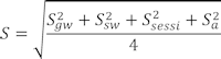
2.1 Overview. The HRS site score (S) is the result of an evaluation of four pathways:
- Ground Water Migration (Sgw).
- Surface Water Migration (Ssw).
- Soil Exposure and Subsurface Intrusion (Ssessi).
- Air Migration (Sa).
The ground water and air migration pathways use single threat evaluations, while the surface water migration and soil exposure and subsurface intrusion pathways use multiple threat evaluations. Three threats are evaluated for the surface water migration pathway: Drinking water, human food chain, and environmental. These threats are evaluated for two separate migration components—overland/flood migration and ground water to surface water migration. Two components are evaluated for the soil exposure and subsurface intrusion pathway: Soil exposure and subsurface intrusion. The soil exposure component evaluates two threats: Resident population and nearby population, and the subsurface intrusion component is a single threat evaluation.
The HRS is structured to provide a parallel evaluation for each of these pathways, components, and threats. This section focuses on these parallel evaluations, starting with the calculation of the HRS site score and the individual pathway scores.
2.1.1 Calculation of HRS site score. Scores are first calculated for the individual pathways as specified in sections 2 through 7 and then are combined for the site using the following root-mean-square equation to determine the overall HRS site score, which ranges from 0 to 100:
2.1.2 Calculation of pathway score. Table 2-1, which is based on the air migration pathway, illustrates the basic parameters used to calculate a pathway score. As Table 2-1 shows, each pathway (component or threat) score is the product of three “factor categories”: Likelihood of release, waste characteristics, and targets. (The soil exposure and subsurface intrusion pathway uses likelihood of exposure rather than likelihood of release.) Each of the three factor categories contains a set of factors that are assigned numerical values and combined as specified in sections 2 through 7. The factor values are rounded to the nearest integer, except where otherwise noted.
2.1.3 Common evaluations. Evaluations common to all four HRS pathways include:
- Characterizing sources.
- Identifying sources (and, for the soil exposure and subsurface intrusion pathway, areas of observed contamination, areas of observed exposure and/or areas of subsurface contamination [see sections 5.1.0 and 5.2.0])
- Identifying hazardous substances associated with each source (or area of observed contamination, or observed exposure, or subsurface contamination).
- Identifying hazardous substances available to a pathway.
| Factor category | Maximum value | Value assigned |
|---|---|---|
| Likelihood of Release | ||
| 1. Observed Release | 550 | |
| 2. Potential to Release | 500 | |
| 3. Likelihood of Release (higher of lines 1 and 2) | 550 | |
| Waste Characteristics | ||
| 4. Toxicity/Mobility | (a) | |
| 5. Hazardous Waste Quantity | (a) | |
| 6. Waste Characteristics | 100 | |
| Targets | ||
| 7. Nearest Individual | ||
| 7a. Level I | 50 | |
| 7b. Level II | 45 | |
| 7c. Potential Contamination | 20 | |
| 7d. Nearest Individual (higher of lines 7a, 7b, or 7c) | 50 | |
| 8. Population | (b) | |
| 8a. Level I | (b) | |
| 8b. Level II | (b) | |
| 8c. Potential Contamination | (b) | |
| 8d. Total Population (lines 8a+8b+8c) | ||
| 9. Resources | 5 | |
| 10. Sensitive Environments | (b) | |
| 10a. Actual Contamination | (b) | |
| 10b. Potential Environments | (b) | |
| 10c. Sensitive Environments (lines 10a+10b) | (b) | |
| 11. Targets (lines 7d+8d+9+10c) | (b) | |
| 12. Pathway Score is the product of Likelihood of Release, Waste Characteristics, and Targets, divided by 82,500. Pathway scores are limited to a maximum of 100 points | ||
| a Maximum value applies to waste characteristics category. The product of lines 4 and 5 is used in Table 2-7 to derive the value for the waste characteristics factor category.
b There is no limit to the human population or sensitive environments factor values. However, the pathway score based solely on sensitive environments is limited to a maximum of 60 points. | ||
- Scoring likelihood of release (or likelihood of exposure) factor category.
- Scoring observed release (or observed exposure or observed contamination).
- Scoring potential to release when there is no observed release.
- Scoring waste characteristics factor category.
- Evaluating toxicity.
- Combining toxicity with mobility, persistence, degradation and/or bioaccumulation (or ecosystem bioaccumulation) potential, as appropriate to the pathway (component or threat).
- Evaluating hazardous waste quantity.
- Combining hazardous waste quantity with the other waste characteristics factors.
- Determining waste characteristics factor category value.
- Evaluating toxicity.
- Scoring targets factor category.
- Determining level of contamination for targets.
These evaluations are essentially identical for the three migration pathways (ground water, surface water, and air). However, the evaluations differ in certain respects for the soil exposure and subsurface intrusion pathway.
Section 7 specifies modifications that apply to each pathway when evaluating sites containing radioactive substances.
Section 2 focuses on evaluations common at the pathway, component, and threat levels. Note that for the ground water and surface water migration pathways, separate scores are calculated for each aquifer (see section 3.0) and each watershed (see sections 4.1.1.3 and 4.2.1.5) when determining the pathway scores for a site. Although the evaluations in section 2 do not vary when different aquifers or watersheds are scored at a site, the specific factor values (for example, observed release, hazardous waste quantity, toxicity/mobility) that result from these evaluations can vary by aquifer and by watershed at the site. This can occur through differences both in the specific sources and targets eligible to be evaluated for each aquifer and watershed and in whether observed releases can be established for each aquifer and watershed. Such differences in scoring at the aquifer and watershed level are addressed in sections 3 and 4, not section 2.
2.2 Characterize sources. Source characterization includes identification of the following:
- Sources (and areas of observed contamination, areas of observed exposure, or areas of subsurface contamination) at the site.
- Hazardous substances associated with these sources (or areas of observed contamination, areas of observed exposure, or areas of subsurface contamination).
- Pathways potentially threatened by these hazardous substances.
Table 2-2 presents a sample worksheet for source characterization.
2.2.1 Identify sources. For the three migration pathways, identify the sources at the site that contain hazardous substances. Identify the migration pathway(s) to which each source applies. For the soil exposure and subsurface intrusion pathway, identify areas of observed contamination, areas of observed exposure, and/or areas of subsurface contamination at the site (see sections 5.1.0 and 5.2.0).
Table 2-2—Sample Source Characterization Worksheet
Source: __
A. Source dimensions and hazardous waste quantity.
Hazardous constituent quantity: __
Hazardous wastestream quantity: __
Volume: __
Area: __
Area of observed contamination: __
Area of observed exposure: __
Area of subsurface contamination: __
B. Hazardous substances associated with the source.
| Hazardous substance | Available to pathway | ||||||||
| Air | Ground Water (GW) | Surface Water (SW) | Soil Exposure/Subsurface Intrusion (SESSI) | ||||||
| Gas | Particulate | Overland/flood | GW to SW | Soil exposure | Subsurface Intrusion | ||||
| Resident | Nearby | Area of observed exposure | Area of subsurface contamination | ||||||
2.2.2 Identify hazardous substances associated with a source. For each of the three migration pathways, consider those hazardous substances documented in a source (for example, by sampling, labels, manifests, oral or written statements) to be associated with that source when evaluating each pathway. In some instances, a hazardous substance can be documented as being present at a site (for example, by labels, manifests, oral or written statements), but the specific source(s) containing that hazardous substance cannot be documented. For the three migration pathways, in those instances when the specific source(s) cannot be documented for a hazardous substance, consider the hazardous substance to be present in each source at the site, except sources for which definitive information indicates that the hazardous substance was not or could not be present.
For an area of observed contamination in the soil exposure component of the soil exposure and subsurface intrusion pathway, consider only those hazardous substances that meet the criteria for observed contamination for that area (see section 5.1.0) to be associated with that area when evaluating the pathway.
For an area of observed exposure or area of subsurface contamination (see section 5.2.0) in the subsurface intrusion component of the soil exposure and subsurface intrusion pathway, consider only those hazardous substances that:
- Meet the criteria for observed exposure, or
- Meet the criteria for observed release in an area of subsurface contamination and have a vapor pressure greater than or equal to one torr or a Henry's constant greater than or equal to 10−5 atm-m3/mol, or
- Meet the criteria for an observed release in a structure within, or in a sample from below, an area of observed exposure and have a vapor pressure greater than or equal to one torr or a Henry's constant greater than or equal to 10−5 atm-m3/mol.
2.2.3 Identify hazardous substances available to a pathway. In evaluating each migration pathway, consider the following hazardous substances available to migrate from the sources at the site to the pathway:
- Ground water migration.
- Hazardous substances that meet the criteria for an observed release (see section 2.3) to ground water.
- All hazardous substances associated with a source with a ground water containment factor value greater than 0 (see section 3.1.2.1).
- Surface water migration—overland/flood component.
- Hazardous substances that meet the criteria for an observed release to surface water in the watershed being evaluated.
- All hazardous substances associated with a source with a surface water containment factor value greater than 0 for the watershed (see sections 4.1.2.1.2.1.1 and 4.1.2.1.2.2.1).
- Surface water migration—ground water to surface water component.
- Hazardous substances that meet the criteria for an observed release to ground water.
- All hazardous substances associated with a source with a ground water containment factor value greater than 0 (see sections 4.2.2.1.2 and 3.1.2.1).
- Air migration.
- Hazardous substances that meet the criteria for an observed release to the atmosphere.
- All gaseous hazardous substances associated with a source with a gas containment factor value greater than 0 (see section 6.1.2.1.1).
- All particulate hazardous substances associated with a source with a particulate containment factor value greater than 0 (see section 6.1.2.2.1).
- For each migration pathway, in those instances when the specific source(s) containing the hazardous substance cannot be documented, consider that hazardous substance to be available to migrate to the pathway when it can be associated (see section 2.2.2) with at least one source having a containment factor value greater than 0 for that pathway.
In evaluating the soil exposure and subsurface intrusion pathway, consider the following hazardous substances available to the pathway:
- Soil exposure component—resident population threat.
- All hazardous substances that meet the criteria for observed contamination at the site (see section 5.1.0).
- Soil exposure component—nearby population threat.
- All hazardous substances that meet the criteria for observed contamination at areas with an attractiveness/accessibility factor value greater than 0 (see section 5.1.2.1.1).
- Subsurface intrusion component.
- All hazardous substances that meet the criteria for observed exposure at the site (see section 5.2.0).
- All hazardous substances with a vapor pressure greater than or equal to one torr or a Henry's constant greater than or equal to 10−5 atm-m3/mol that meet the criteria for an observed release in an area of subsurface contamination (see section 5.2.0).
- All hazardous substances that meet the criteria for an observed release in a structure within, or in a sample from below, an area of observed exposure (see section 5.2.0).
2.3 Likelihood of release. Likelihood of release is a measure of the likelihood that a waste has been or will be released to the environment. The likelihood of release factor category is assigned the maximum value of 550 for a migration pathway whenever the criteria for an observed release are met for that pathway. If the criteria for an observed release are met, do not evaluate potential to release for that pathway. When the criteria for an observed release are not met, evaluate potential to release for that pathway, with a maximum value of 500. The evaluation of potential to release varies by migration pathway (see sections 3, 4 and 6).
Establish an observed release either by direct observation of the release of a hazardous substance into the media being evaluated (for example, surface water) or by chemical analysis of samples appropriate to the pathway being evaluated (see sections 3, 4 and 6). The minimum standard to establish an observed release by chemical analysis is analytical evidence of a hazardous substance in the media significantly above the background level. Further, some portion of the release must be attributable to the site. Use the criteria in Table 2-3 as the standard for determining analytical significance. (The criteria in Table 2-3 are also used in establishing observed contamination for the soil exposure component and for establishing areas of observed exposure and areas of subsurface contamination in the subsurface intrusion component of the soil exposure and subsurface intrusion pathway, see section 5.1.0 and section 5.2.0). Separate criteria apply to radionuclides (see section 7.1.1).
| Sample Measurement < Sample Quantitation Limit. a |
| No observed release is established. |
| Sample Measurement ≥ Sample Quantitation Limit. a |
| An observed release is established as follows: |
|
|
| a If the sample quantitation limit (SQL) cannot be established, determine if there is an observed release as follows: |
|
|
2.4 Waste characteristics. The waste characteristics factor category includes the following factors: Hazardous waste quantity, toxicity, and as appropriate to the pathway or threat being evaluated, mobility, persistence, degradation, and/or bioaccumulation (or ecosystem bioaccumulation) potential.
2.4.1 Selection of substance potentially posing greatest hazard. For all pathways (components and threats), select the hazardous substance potentially posing the greatest hazard for the pathway (component or threat) and use that substance in evaluating the waste characteristics category of the pathway (component or threat). For the three migration pathways (and threats), base the selection of this hazardous substance on the toxicity factor value for the substance, combined with its mobility, persistence, and/or bioaccumulation (or ecosystem bioaccumulation) potential factor values, as applicable to the migration pathway (or threat). For the soil exposure component of the soil exposure and subsurface intrusion pathway, base the selection on the toxicity factor alone. For the subsurface intrusion component of the soil exposure and subsurface intrusion pathway, base the selection on the toxicity factor value for the substance, combined with its degradation factor value. Evaluation of the toxicity factor is specified in section 2.4.1.1. Use and evaluation of the mobility, persistence, degradation, and/or bioaccumulation (or ecosystem bioaccumulation) potential factors vary by pathway (component or threat) and are specified under the appropriate pathway (component or threat) section. Section 2.4.1.2 identifies the specific factors that are combined with toxicity in evaluating each pathway (component or threat).
2.4.1.1 Toxicity factor. Evaluate toxicity for those hazardous substances at the site that are available to the pathway being scored. For all pathways and threats, except the surface water environmental threat, evaluate human toxicity as specified below. For the surface water environmental threat, evaluate ecosystem toxicity as specified in section 4.1.4.2.1.1.
Establish human toxicity factor values based on quantitative dose-response parameters for the following three types of toxicity:
- Cancer—Use slope factors (also referred to as cancer potency factors) combined with weight-of-evidence ratings for carcinogenicity for all exposure routes except inhalation. Use inhalation unit risk (IUR) for inhalation exposure. If an inhalation unit risk or a slope factor is not available for a substance, use its ED10 value to estimate a slope factor as follows:
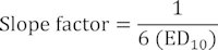
- Noncancer toxicological responses of chronic exposure—use reference dose (RfD) or reference concentration (RfC) values as applicable.
- Noncancer toxicological responses of acute exposure—use acute toxicity parameters, such as the LD50.
Assign human toxicity factor values to a hazardous substance using Table 2-4, as follows:
- If RfD/RfC and slope factor/inhalation unit risk values are available for the hazardous substance, assign the substance a value from Table 2-4 for each. Select the higher of the two values assigned and use it as the overall toxicity factor value for the hazardous substance.
- If either an RfD/RfC or slope factor/inhalation unit risk value is available, but not both, assign the hazardous substance an overall toxicity factor value from Table 2-4 based solely on the available value (RfD/RfC or slope factor/inhalation unit risk).
- If neither an RfD/RfC nor slope factor/inhalation unit risk value is available, assign the hazardous substance an overall toxicity factor value from Table 2-4 based solely on acute toxicity. That is, consider acute toxicity in Table 2-4 only when both RfD/RfC and slope factor/IUR values are not available.
- If neither an RfD/RfC, nor slope factor/inhalation unit risk, nor acute toxicity value is available, assign the hazardous substance an overall toxicity factor value of 0 and use other hazardous substances for which information is available in evaluating the pathway.
| Assigned value | |
|---|---|
| Chronic Toxicity (Human) | |
| Reference dose (RfD) (mg/kg-day): | |
| RfD < 0.0005 | 10,000 |
| 0.0005 ≤ RfD < 0.005 | 1,000 |
| 0.005 ≤ RfD < 0.05 | 100 |
| 0.05 ≤ RfD < 0.5 | 10 |
| 0.5 ≤ RfD | 1 |
| RfD not available | 0 |
| Reference concentration (RfC) (mg/m3): | |
| RfC < 0.0001 | 10,000 |
| 0.0001 ≤ RfC < 0.006 | 1,000 |
| 0.006 ≤ RfC < 0.2 | 100 |
| 0.2 ≤ RfC < 2.0 | 10 |
| 2.0 ≤ RfC | 1 |
| RfC not available | 0 |
| Carcinogenicity (human) | |||
|---|---|---|---|
| A or Carcinogenic to humans | B or Likely to be carcinogenic to humans | C or Suggestive evidence of carcinogenic potential | Assigned value |
| Weight-of-evidence/Slope factor (mg/kg-day) | |||
| 0.5 ≤ SFb | 5 ≤ SF | 50 ≤ SF | 10,000 |
| 0.05 ≤ SF < 0.5 | 0.5 ≤ SF < 5 | 5 ≤ SF < 50 | 1,000 |
| SF < 0.05 | 0.05 ≤ SF < 0.5 | 0.5 ≤ SF < 5 | 100 |
| SF < 0.05 | SF < 0.5 | 10 | |
| Slope factor not available | Slope factor not available | Slope factor not available | 0 |
| Weight-of-evidence/Inhalation unit risk (μg/m) | |||
| 0.00004 ≤ IURc | 0.0004 ≤ IUR | 0.004 ≤ IUR | 10,000 |
| 0.00001 ≤ IUR < 0.00004 | 0.0001 ≤ IUR < 0.0004 | 0.001 ≤ IUR < 0.004 | 1,000 |
| IUR < 0.00001 | 0.00001 ≤ IUR < 0.0001 | 0.0001 ≤ IUR < 0.001 | 100 |
| < 0.00001 | IUR < 0.0001 | 10 | |
| Inhalation unit risk not available | Inhalation unit risk not available | Inhalation unit risk not available | 0 |
| a A, B, and C, as well as Carcinogenic to humans, Likely to be carcinogenic to humans, and Suggestive evidence of carcinogenic potential refer to weight-of-evidence categories. Assign substances with a weight-of-evidence category of D (inadequate evidence of carcinogenicity) or E (evidence of lack of carcinogenicity), as well as inadequate information to assess carcinogenic potential and not likely to be carcinogenic to humans a value of 0 for carcinogenicity.
b SF = Slope factor. c IUR = Inhalation Unit Risk. | |||
| Acute Toxicity (human) | ||||
|---|---|---|---|---|
| Oral LD (mg/kg) | Dermal LD (mg/kg) | Dust or mist LC (mg/l) | Gas or vapor LC (ppm) | Assigned value |
| LD < 5 | LD < 2 | LC < 0.2 | LC < 20 | 1,000 |
| 5 ≤ LD < 50 | 2 ≤ LD < 20 | 0.2 ≤ LC < 2 | 20 ≤ LC <200 | 100 |
| 50 ≤ LD < 500 | 20 ≤ LD < 200 | 2 ≤ LC <20 | 200 ≤ LC <2,000 | 10 |
| 500 ≤ LD | 200 ≤ LD | 20 ≤ LC | 2,000 ≤ LC | 1 |
| LD not available | LD not available | LC not available | LC not available | 0 |
If a toxicity factor value of 0 is assigned to all hazardous substances available to a particular pathway (that is, insufficient toxicity data are available for evaluating all the substances), use a default value of 100 as the overall human toxicity factor value for all hazardous substances available to the pathway. For hazardous substances having usable toxicity data for multiple exposure routes (for example, inhalation and ingestion), consider all exposure routes and use the highest assigned value, regardless of exposure route, as the toxicity factor value. For HRS purposes, assign both asbestos and lead (and its compounds) a human toxicity factor value of 10,000.
Separate criteria apply for assigning factor values for human toxicity and ecosystem toxicity for radionuclides (see sections 7.2.1 and 7.2.2).
2.4.1.2 Hazardous substance selection. For each hazardous substance evaluated for a migration pathway (or threat), combine the human toxicity factor value (or ecosystem toxicity factor value) for the hazardous substance with a mobility, persistence, and/or bioaccumulation (or ecosystem bioaccumulation) potential factor value as follows:
- Ground water migration.
- Determine a combined human toxicity/mobility factor value for the hazardous substance (see section 3.2.1).
- Surface water migration—overland/flood migration component.
- Determine a combined human toxicity/persistence factor value for the hazardous substance for the drinking water threat (see section 4.1.2.2.1).
- Determine a combined human toxicity/persistence/bioaccumulation factor value for the hazardous substance for the human food chain threat (see section 4.1.3.2.1).
- Determine a combined ecosystem toxicity/persistence/bioaccumulation factor value for the hazardous substance for the environmental threat (see section 4.1.4.2.1).
- Surface water migration—ground water to surface water migration component.
- Determine a combined human toxicity/mobility/persistence factor value for the hazardous substance for the drinking water threat (see section 4.2.2.2.1).
- Determine a combined human toxicity/mobility/persistence/bioaccumulation factor value for the hazardous substance for the human food chain threat (see section 4.2.3.2.1).
- Determine a combined ecosystem toxicity/mobility/persistence/bioaccumulation factor value for the hazardous substance for the environmental threat (see section 4.2.4.2.1).
- Air migration.
- Determine a combined human toxicity/mobility factor value for the hazardous substance (see section 6.2.1).
Determine each combined factor value for a hazardous substance by multiplying the individual factor values appropriate to the pathway (or threat). For each migration pathway (or threat) being evaluated, select the hazardous substance with the highest combined factor value and use that substance in evaluating the waste characteristics factor category of the pathway (or threat).
For the soil exposure and subsurface intrusion pathway, determine toxicity and toxicity/degradation factor values as follows:
- Soil exposure and subsurface intrusion—soil exposure component.
- Select the hazardous substance with the highest human toxicity factor value from among the substances that meet the criteria for observed contamination for the threat evaluated and use that substance in evaluating the waste characteristics factor category (see section 5.1.1.2.1).
- Soil exposure and subsurface intrusion—subsurface intrusion component.
- Determine a combined human toxicity/degradation factor value for each hazardous substance being evaluated that:
- Meets the criteria for observed exposure, or
- Meets the criteria for observed release in an area of subsurface contamination and has a vapor pressure greater than or equal to one torr or a Henry's constant greater than or equal to 10−5 atm-m 3 /mol, or
- Meets the criteria for an observed release in a structure within, or in a sample from below, an area of observed exposure and has a vapor pressure greater than or equal to one torr or a Henry's constant greater than or equal to 10−5 atm-m3/mol.
- Select the hazardous substance with the highest combined factor value and use that substance in evaluating the waste characteristics factor category (see sections 5.2.1.2.1 and 5.2.1.2).
- Determine a combined human toxicity/degradation factor value for each hazardous substance being evaluated that:
2.4.2 Hazardous waste quantity. Evaluate the hazardous waste quantity factor by first assigning each source (or area of observed contamination, area of observed exposure, or area of subsurface contamination) a source hazardous waste quantity value as specified below. Sum these values to obtain the hazardous waste quantity factor value for the pathway being evaluated.
In evaluating the hazardous waste quantity factor for the three migration pathways, allocate hazardous substances and hazardous wastestreams to specific sources in the manner specified in section 2.2.2, except: Consider hazardous substances and hazardous wastestreams that cannot be allocated to any specific source to constitute a separate “unallocated source” for purposes of evaluating only this factor for the three migration pathways. Do not, however, include a hazardous substance or hazardous wastestream in the unallocated source for a migration pathway if there is definitive information indicating that the substance or wastestream could only have been placed in sources with a containment factor value of 0 for that migration pathway.In evaluating the hazardous waste quantity factor for the soil exposure component of the soil exposure and subsurface intrusion pathway, allocate to each area of observed contamination only those hazardous substances that meet the criteria for observed contamination for that area of observed contamination and only those hazardous wastestreams that contain hazardous substances that meet the criteria for observed contamination for that area of observed contamination. Do not consider other hazardous substances or hazardous wastestreams at the site in evaluating this factor for the soil exposure component of the soil exposure and subsurface intrusion pathway.
In evaluating the hazardous waste quantity factor for the subsurface intrusion component of the soil exposure and subsurface intrusion pathway, allocate to each area of observed exposure or area of subsurface contamination only those hazardous substances and hazardous wastestreams that contain hazardous substances that:
- Meet the criteria for observed exposure, or
- Meet the criteria for observed release in an area of subsurface contamination and have a vapor pressure greater than or equal to one torr or a Henry's constant greater than or equal to 10−5 atm-m3/mol, or
- Meet the criteria for an observed release in a structure within, or in a sample from below, an area of observed exposure and have a vapor pressure greater than or equal to one torr or a Henry's constant greater than or equal to 10−5 atm-m3/mol.
Do not consider other hazardous substances or hazardous wastestreams at the site in evaluating this factor for the subsurface intrusion component of the soil exposure and subsurface intrusion pathway. When determining the hazardous waste quantity for multi-subunit structures, use the procedures identified in section 5.2.1.2.2.
2.4.2.1 Source hazardous waste quantity. For each of the three migration pathways, assign a source hazardous waste quantity value to each source (including the unallocated source) having a containment factor value greater than 0 for the pathway being evaluated. Consider the unallocated source to have a containment factor value greater than 0 for each migration pathway.
For the soil exposure component of the soil exposure and subsurface intrusion pathway, assign a source hazardous waste quantity value to each area of observed contamination, as applicable to the threat being evaluated.
For the subsurface intrusion component of the soil exposure and subsurface intrusion pathway, assign a source hazardous waste quantity value to each regularly occupied structure within an area of observed exposure or an area of subsurface contamination that has a structure containment factor value greater than 0. If sufficient data is available and state of the science shows there is no unacceptable risk due to subsurface intrusion into a regularly occupied structure located within an area of subsurface contamination, that structure can be excluded from the area of subsurface contamination.
For determining all hazardous waste quantity calculations except for an unallocated source or an area of subsurface contamination, evaluate using the following four measures in the following hierarchy:
- Hazardous constituent quantity.
- Hazardous wastestream quantity.
- Volume.
- Area.
For the unallocated source, use only the first two measures. For an area of subsurface contamination, evaluate non-radioactive hazardous substances using only the last two measures and evaluate radioactive hazardous substances using hazardous wastestream quantity only. See also section 7.0 regarding the evaluation of radioactive substances.
Separate criteria apply for assigning a source hazardous waste quantity value for radionuclides (see section 7.2.5).
2.4.2.1.1 Hazardous constituent quantity. Evaluate hazardous constituent quantity for the source (or area of observed contamination) based solely on the mass of CERCLA hazardous substances (as defined in CERCLA section 101(14), as amended) allocated to the source (or area of observed contamination), except:
- For a hazardous waste listed pursuant to section 3001 of the Solid Waste Disposal Act, as amended by the Resource Conservation and Recovery Act of 1976 (RCRA), 42 U.S.C. 6901 et seq., determine its mass for the evaluation of this measure as follows:
- If the hazardous waste is listed solely for Hazard Code T (toxic waste), include only the mass of constituents in the hazardous waste that are CERCLA hazardous substances and not the mass of the entire hazardous waste.
- If the hazardous waste is listed for any other Hazard Code (including T plus any other Hazard Code), include the mass of the entire hazardous waste.
- For a RCRA hazardous waste that exhibits the characteristics identified under section 3001 of RCRA, as amended, determine its mass for the evaluation of this measure as follows:
- If the hazardous waste exhibits only the characteristic of toxicity (or only the characteristic of EP toxicity), include only the mass of constituents in the hazardous waste that are CERCLA hazardous substances and not the mass of the entire hazardous waste.
- If the hazardous waste exhibits any other characteristic identified under section 3001 (including any other characteristic plus the characteristic of toxicity [or the characteristic of EP toxicity]), include the mass of the entire hazardous waste.
Based on this mass, designated as C, assign a value for hazardous constituent quantity as follows:
- For the migration pathways, assign the source a value for hazardous constituent quantity using the Tier A equation of Table 2-5.
- For the soil exposure and subsurface intrusion pathway—soil exposure component, assign the area of observed contamination a value using the Tier A equation of Table 5-2 (section 5.1.1.2.2).
- For the soil exposure and subsurface intrusion pathway—subsurface intrusion component, assign the area of observed exposure a value using the Tier A equation of Table 5-19 (section 5.2.1.2.2).
If the hazardous constituent quantity for the source (or area of observed contamination or area of observed exposure) is adequately determined (that is, the total mass of all CERCLA hazardous substances in the source and releases from the source [or in the area of observed contamination or area of observed exposure] is known or is estimated with reasonable confidence), do not evaluate the other three measures discussed below. Instead assign these other three measures a value of 0 for the source (or area of observed contamination or area of observed exposure) and proceed to section 2.4.2.1.5.
If the hazardous constituent quantity is not adequately determined, assign the source (or area of observed contamination or area of observed exposure) a value for hazardous constituent quantity based on the available data and proceed to section 2.4.2.1.2.
| Tier | Measure | Units | Equation for assigning valuea |
|---|---|---|---|
| A | Hazardous constituent quantity (C) | lb | C. |
| B b | Hazardous wastestream quantity (W) | lb | W/5,000. |
| C b | Volume (V) | ||
| Landfill | yd3 | V/2,500. | |
| Surface impoundment | yd3 | V/2.5. | |
| Surface impoundment (buried/backfilled) | yd3 | V/2.5. | |
| Drumsc | gallon | V/500. | |
| Tanks and containers other than drums | yd3 | V/2.5. | |
| Contaminated soil | yd3 | V/2,500. | |
| Pile | yd3 | V/2.5. | |
| Other | yd3 | V/2.5. | |
| D b | Area (A) | ||
| Landfill | ft2 | A/3,400. | |
| Surface impoundment | ft2 | A/13. | |
| Surface impoundment (buried/backfilled) | ft2 | A/13. | |
| Land treatment | ft2 | A/270. | |
| Piled | ft2 | A/13. | |
| Contaminated soil | ft2 | A/34,000. | |
| a Do not round to nearest integer. b Convert volume to mass when necessary: 1 ton = 2,000 pounds = 1 cubic yard = 4 drums = 200 gallons. c If actual volume of drums is unavailable, assume 1 drum=50 gallons. d Use land surface area under pile, not surface area of pile. | |||
2.4.2.1.2 Hazardous wastestream quantity. Evaluate hazardous wastestream quantity for the source (or area of observed contamination or area of observed exposure) based on the mass of hazardous wastestreams plus the mass of any additional CERCLA pollutants and contaminants (as defined in CERCLA section 101[33], as amended) that are allocated to the source (or area of observed contamination or area of observed exposure). For a wastestream that consists solely of a hazardous waste listed pursuant to section 3001 of RCRA, as amended or that consists solely of a RCRA hazardous waste that exhibits the characteristics identified under section 3001 of RCRA, as amended, include the mass of that entire hazardous waste in the evaluation of this measure.
Based on this mass, designated as W, assign a value for hazardous wastestream quantity as follows:
- For the migration pathways, assign the source a value for hazardous wastestream quantity using the Tier B equation of Table 2-5.
- For the soil exposure and subsurface intrusion pathway—soil exposure component, assign the area of observed contamination a value using the Tier B equation of Table 5-2 (section 5.1.1.2.2).
- For the soil exposure and subsurface intrusion pathway—subsurface intrusion component, assign the area of observed exposure a value using the Tier B equation of Table 5-19 (section 5.2.1.2.2).
Do not evaluate the volume and area measures described below if the source is the unallocated source or if the following condition applies:
- The hazardous wastestream quantity for the source (or area of observed contamination or area of observed exposure) is adequately determined—that is, total mass of all hazardous wastestreams and CERCLA pollutants and contaminants for the source and releases from the source (or for the area of observed contamination) is known or is estimated with reasonable confidence.
If the source is the unallocated source or if this condition applies, assign the volume and area measures a value of 0 for the source (or area of observed contamination) and proceed to section 2.4.2.1.5. Otherwise, assign the source (or area of observed contamination) a value for hazardous wastestream quantity based on the available data and proceed to section 2.4.2.1.3.
2.4.2.1.3 Volume. Evaluate the volume measure using the volume of the source (or the volume of the area of observed contamination, area of observed exposure, or area of subsurface contamination). For the soil exposure and subsurface intrusion pathway, restrict the use of the volume measure to those areas of observed contamination, areas of observed exposure, or areas of subsurface contamination as specified in sections 5.1.1.2.2 and 5.2.1.2.2.
Based on the volume, designated as V, assign a value to the volume measure as follows:
- For the migration pathways, assign the source a value for volume using the appropriate Tier C equation of Table 2-5.
- For the soil exposure and subsurface intrusion pathway—soil exposure component, assign the area of observed contamination a value for volume using the appropriate Tier C equation of Table 5-2 (section 5.1.1.2.2).
- For the soil exposure and subsurface intrusion pathway—subsurface intrusion component, assign the value based on the volume of the regularly occupied structures within the area of observed exposure or area of subsurface contamination using the Tier C equation of Table 5-19 (section 5.2.1.2.2).
If the volume of the source (or volume of the area of observed contamination, area of observed exposure, or area of subsurface contamination, if applicable) can be determined, do not evaluate the area measure. Instead, assign the area measure a value of 0 and proceed to section 2.4.2.1.5. If the volume cannot be determined (or is not applicable for the soil exposure and subsurface intrusion pathway), assign the source (or area of observed contamination, area of observed exposure, or area of subsurface contamination) a value of 0 for the volume measure and proceed to section 2.4.2.1.4.
2.4.2.1.4 Area. Evaluate the area measure using the area of the source (or the area of the area of observed contamination, area of observed exposure, or area of subsurface contamination). Based on this area, designated as A, assign a value to the area measure as follows:
- For the migration pathways, assign the source a value for area using the appropriate Tier D equation of Table 2-5.
- For the soil exposure and subsurface intrusion pathway—soil exposure component, assign the area of observed contamination a value for area using the appropriate Tier D equation of Table 5-2 (section 5.1.1.2.2).
- For the soil exposure and subsurface intrusion pathway—subsurface intrusion component, assign a value based on the area of regularly occupied structures within the area of observed exposure or area of subsurface contamination using the Tier D equation of Table 5-19 (section 5.2.1.2.2).
2.4.2.1.5 Calculation of source hazardous waste quantity value. Select the highest of the values assigned to the source (or areas of observed contamination, areas of observed exposure, or areas of subsurface contamination) for the hazardous constituent quantity, hazardous wastestream quantity, volume, and area measures. Assign this value as the source hazardous waste quantity value. Do not round to the nearest integer.
2.4.2.2 Calculation of hazardous waste quantity factor value. Sum the source hazardous waste quantity values assigned to all sources (including the unallocated source) or areas of observed contamination, areas of observed exposure, or areas of subsurface contamination for the pathway being evaluated and round this sum to the nearest integer, except: If the sum is greater than 0, but less than 1, round it to 1. Based on this value, select a hazardous waste quantity factor value for the pathway from Table 2-6.
| Hazardous waste quantity value | Assigned value |
|---|---|
| 0 | 0 |
| 1 a to 100 | b 1 |
| Greater than 100 to 10,000 | 100 |
| Greater than 10,000 to 1,000,000 | 10,000 |
| Greater than 1,000,000 | 1,000,000 |
| a If the hazardous waste quantity value is greater than 0, but less than 1, round it to 1 as specified in text. | |
| b For the pathway, if hazardous constituent quantity is not adequately determined, assign a value as specified in the text; do not assign the value of 1. | |
For a migration pathway, if the hazardous constituent quantity is adequately determined (see section 2.4.2.1.1) for all sources (or all portions of sources and releases remaining after a removal action), assign the value from Table 2-6 as the hazardous waste quantity factor value for the pathway. If the hazardous constituent quantity is not adequately determined for one or more sources (or one or more portions of sources or releases remaining after a removal action) assign a factor value as follows:
- If any target for that migration pathway is subject to Level I or Level II concentrations (see section 2.5), assign either the value from Table 2-6 or a value of 100, whichever is greater, as the hazardous waste quantity factor value for that pathway.
- If none of the targets for that pathway is subject to Level I or Level II concentrations, assign a factor value as follows:
- If there has been no removal action, assign either the value from Table 2-6 or a value of 10, whichever is greater, as the hazardous waste quantity factor value for that pathway.
- If there has been a removal action:
- Determine values from Table 2-6 with and without consideration of the removal action.
- If the value that would be assigned from Table 2-6 without consideration of the removal action would be 100 or greater, assign either the value from Table 2-6 with consideration of the removal action or a value of 100, whichever is greater, as the hazardous waste quantity factor value for the pathway.
- If the value that would be assigned from Table 2-6 without consideration of the removal action would be less than 100, assign a value of 10 as the hazardous waste quantity factor value for the pathway.
For the soil exposure component of the soil exposure and subsurface intrusion pathway, if the hazardous constituent quantity is adequately determined for all areas of observed contamination, assign the value from Table 2-6 as the hazardous waste quantity factor value. If the hazardous constituent quantity is not adequately determined for one or more areas of observed contamination, assign either the value from Table 2-6 or a value of 10, whichever is greater, as the hazardous waste quantity factor value.
For the subsurface intrusion component of the soil exposure and subsurface intrusion pathway, if the hazardous constituent quantity is adequately determined for all areas of observed exposure, assign the value from Table 2-6 as the hazardous waste quantity factor value. If the hazardous constituent quantity is not adequately determined for one or more areas of observed exposure, assign either the value from Table 2-6 or assign a factor value as follows:
- If any target for the subsurface intrusion component is subject to Level I or Level II concentrations (see section 2.5), assign either the value from Table 2-6 or a value of 100, whichever is greater, as the hazardous waste quantity factor value for this component.
- If none of the targets for the subsurface intrusion component is subject to Level I or Level II concentrations and if there has been a removal or other temporary response action that does not permanently interrupt target exposure form subsurface intrusion, assign a factor value as follows:
- Determine the values from Table 2-6 with and without consideration of the removal or other temporary response action.
- If the value that would be assigned from Table 2-6 without consideration of the removal or other temporary response action would be 100 or greater, assign either the value from Table 2-6 with consideration of the removal action or a value of 100, whichever is greater, as the hazardous waste quantity factor value for the component.
- If the value that would be assigned from Table 2-6 without consideration of the removal or other temporary response action would be less than 100, assign a value of 10 as the hazardous waste quantity factor value for the component.
- Otherwise, if none of the targets for the subsurface intrusion component is subject to Level I or Level II concentrations and there has not been a removal action, assign a value from Table 2-6 or a value of 10, whichever is greater.
2.4.3 Waste characteristics factor category value. Determine the waste characteristics factor category value as specified in section 2.4.3.1 for all pathways and threats, except the surface water-human food chain threat and the surface water-environmental threat. Determine the waste characteristics factor category value for these latter two threats as specified in section 2.4.3.2.
2.4.3.1 Factor category value. For the pathway (component or threat) being evaluated, multiply the toxicity or combined factor value, as appropriate, from section 2.4.1.2 and the hazardous waste quantity factor value from section 2.4.2.2, subject to a maximum product of 1x10 8. Based on this waste characteristics product, assign a waste characteristics factor category value to the pathway (component or threat) from Table 2-7.
| Waste characteristics product | Assigned value |
|---|---|
| 0 | 0 |
| Greater than 0 to less than 10 | 1 |
| 10 to less than 1x10² | 2 |
| 1x10² to less than 1x10³ | 3 |
| 1x10³ to less than 1x10⁴ | 6 |
| 1x10⁴ to less than 1x10⁵ | 10 |
| 1x10⁵ to less than 1x10⁶ | 18 |
| 1x10⁶ to less than 1x10⁷ | 32 |
| 1x10⁷ to less than 1x10⁸ | 56 |
| 1x10⁸ to less than 1x10⁹ | 100 |
| 1x10⁹ to less than 1x10¹⁰ | 180 |
| 1x10¹⁰ to less than 1x10¹¹ | 320 |
| 1x10¹¹ to less than 1x10¹² | 560 |
| 1x10¹² | 1,000 |
2.4.3.2 Factor category value, considering bioaccumulation potential. For the surface water-human food chain threat and the surface water-environmental threat, multiply the toxicity or combined factor value, as appropriate, from section 2.4.1.2 and the hazardous waste quantity factor value from section 2.4.2.2, subject to:
- A maximum product of 1x10¹², and
- A maximum product exclusive of the bioaccumulation (or ecosystem bioaccumulation) potential factor of 1x10⁸.
Based on the total waste characteristics product, assign a waste characteristics factor category value to these threats from Table 2-7.
2.5 Targets. The types of targets evaluated include the following:
- Individual (factor name varies by pathway, component, and threat).
- Human population.
- Resources (these vary by pathway, component, and threat).
- Sensitive environments (included for the surface water migration pathway, air migration pathway, and soil exposure component of the soil exposure and subsurface intrusion pathway).
The factor values that may be assigned to each type of target have the same range for each pathway for which that type of target is evaluated. The factor value for most types of targets depends on whether the target is subject to actual or potential contamination for the pathway and whether the actual contamination is Level I or Level II:
- Actual contamination: Target is associated either with a sampling location that meets the criteria for an observed release (or observed contamination or observed exposure) for the pathway or with an observed release based on direct observation for the pathway (additional criteria apply for establishing actual contamination for the human food chain threat in the surface water migration pathway, see sections 4.1.3.3 and 4.2.3.3). Sections 3 through 6 specify how to determine the targets associated with a sampling location or with an observed release based on direct observation. Determine whether the actual contamination is Level I or Level II as follows:
- Level I:
- Media-specific concentrations for the target meet the criteria for an observed release (or observed contamination or observed exposure) for the pathway and are at or above media-specific benchmark values. These benchmark values (see section 2.5.2) include both screening concentrations and concentrations specified in regulatory limits (such as Maximum Contaminant Level (MCL) values), or
- For the human food chain threat in the surface water migration pathway, concentrations in tissue samples from aquatic human food chain organisms are at or above benchmark values. Such tissue samples may be used in addition to media-specific concentrations only as specified in sections 4.1.3.3 and 4.2.3.3.
- Level II:
- Media-specific concentrations for the target meet the criteria for an observed release (or observed contamination or observed exposure) for the pathway, but are less than media-specific benchmarks. If none of the hazardous substances eligible to be evaluated for the sampling location has an applicable benchmark, assign Level II to the actual contamination at the sampling location, or
- For observed releases or observed exposures based on direct observation, assign Level II to targets as specified in sections 3, 4, 5, and 6, or
- For the human food chain threat in the surface water migration pathway, concentrations in tissue samples from aquatic human food chain organisms, when applicable, are below benchmark values.
- If a target is subject to both Level I and Level II concentrations for a pathway (component or threat), evaluate the target using Level I concentrations for that pathway (component or threat).
- Level I:
- Potential contamination: Target is subject to a potential release (that is, target is not associated with actual contamination for that pathway or threat).
Assign a factor value for individual risk as follows (select the highest value that applies to the pathway, component or threat):
- 50 points if any individual is exposed to Level I concentrations.
- 45 points if any individual is exposed to Level II concentrations.
- Maximum of 20 points if any individual is subject to potential contamination. The value assigned is 20 unless reduced by a distance or dilution weight appropriate to the pathway. Assign factor values for population and sensitive environments as follows:
- Sum Level I targets and multiply by 10. (Level I is not used for sensitive environments in the soil exposure component of the soil exposure and subsurface intrusion and air migration pathways.)
- Sum Level II targets.
- Multiply potential targets in all but the soil exposure and subsurface intrusion pathway by distance or dilution weights appropriate to the pathway, sum, and divide by 10. Distance or dilution weighting accounts for diminishing exposure with increasing distance or dilution within the different pathways. For targets within an area of subsurface contamination in the subsurface intrusion component of the soil exposure and subsurface intrusion pathway, multiply by a weighting factor as directed in section 5.2.1.3.2.3.
- Sum the values for the three levels.
In addition, resource value points are assigned within all pathways for welfare-related impacts (for example, impacts to agricultural land), but do not depend on whether there is actual or potential contamination.
2.5.1 Determination of level of actual contamination at a sampling location. Determine whether Level I concentrations or Level II concentrations apply at a sampling location (and thus to the associated targets) as follows:
- Select the benchmarks applicable to the pathway (component or threat) being evaluated.
- Compare the concentrations of hazardous substances in the sample (or comparable samples) to their benchmark concentrations for the pathway (component or threat), as specified in section 2.5.2.
- Determine which level applies based on this comparison.
- If none of the hazardous substances eligible to be evaluated for the sampling location has an applicable benchmark, assign Level II to the actual contamination at that sampling location for the pathway (component or threat).
In making the comparison, consider only those samples, and only those hazardous substances in the sample, that meet the criteria for an observed release (or observed contamination or observed exposure) for the pathway, except: Tissue samples from aquatic human food chain organisms may also be used as specified in sections 4.1.3.3 and 4.2.3.3 of the surface water-human food chain threat. If any hazardous substance is present in more than one comparable sample for the sampling location, use the highest concentration of that hazardous substance from any of the comparable samples in making the comparisons.
Treat sets of samples that are not comparable separately and make a separate comparison for each such set.
2.5.2 Comparison to benchmarks. Use the following media-specific benchmarks for making the comparisons for the indicated pathway (or threat):
- Maximum Contaminant Level Goals (MCLGs)—ground water migration pathway and drinking water threat in surface water migration pathway. Use only MCLG values greater than 0.
- Maximum Contaminant Levels (MCLs)—ground water migration pathway and drinking water threat in surface water migration pathway.
- Food and Drug Administration Action Level (FDAAL) for fish or shellfish—human food chain threat in surface water migration pathway.
- EPA Ambient Water Quality Criteria (AWQC/National Recommended Water Quality Criteria) for protection of aquatic life—environmental threat in surface water migration pathway.
- EPA Ambient Aquatic Life Advisory Concentrations (AALAC)—environmental threat in surface water migration pathway.
- National Ambient Air Quality Standards (NAAQS)—air migration pathway.
- National Emission Standards for Hazardous Air Pollutants (NESHAPs)—air migration pathway. Use only those NESHAPs promulgated in ambient concentration units.
- Screening concentration for cancer corresponding to that concentration that corresponds to the 10 −6 individual cancer risk for inhalation exposures (air migration pathway or subsurface intrusion component of the soil exposure and subsurface intrusion pathway) or for oral exposures (ground water migration pathway; drinking water and human food chain threats in surface water migration pathway; and soil exposure and subsurface intrusion pathway).
- Screening concentration for noncancer toxicological responses corresponding to the RfC for inhalation exposures (air migration pathway and subsurface intrusion component of the soil exposure and subsurface intrusion pathway) or RfD for oral exposures (ground water migration pathway; drinking water and human food chain threats in surface water migration pathway; and soil exposure and subsurface intrusion pathway).
Select the benchmark(s) applicable to the pathway (component or threat) being evaluated as specified in sections 3 through 6. Compare the concentration of each hazardous substance from the sampling location to its benchmark concentration(s) for that pathway (component or threat). Use only those samples and only those hazardous substances in the sample that meet the criteria for an observed release (or observed contamination or observed exposure) for the pathway, except: Tissue samples from aquatic human food chain organisms may be used as specified in sections 4.1.3.3 and 4.2.3.3. If the concentration of any applicable hazardous substance from any sample equals or exceeds its benchmark concentration, consider the sampling location to be subject to Level I concentrations for that pathway (or threat). If more than one benchmark applies to the hazardous substance, assign Level I if the concentration of the hazardous substance equals or exceeds the lowest applicable benchmark concentration.
If no hazardous substance individually equals or exceeds its benchmark concentration, but more than one hazardous substance either meets the criteria for an observed release (or observed contamination or observed exposure) for the sample (or comparable samples) or is eligible to be evaluated for a tissue sample (see sections 4.1.3.3 and 4.2.3.3), calculate the indices I and J specified below based on these hazardous substances.
For those hazardous substances that are carcinogens (that is, those having either a carcinogen weight-of-evidence classification of A, B, or C or a weight-of-evidence classification of carcinogenic to humans, likely to be carcinogenic to humans, or suggestive evidence of carcinogenic potential), calculate an index I for the sample location as follows:
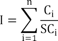
Where:
C i = Concentration of hazardous substance i in sample (or highest concentration of hazardous substance i from among comparable samples).
SC i = Screening concentration for cancer corresponding to that concentration that corresponds to its 10 −6 individual cancer risk for applicable exposure (inhalation or oral) for hazardous substance i.
n = Number of applicable hazardous substances in sample (or comparable samples) that are carcinogens and for which an SC i is available.
For those hazardous substances for which an RfD or RfC is available, calculate an index J for the sample location as follows:
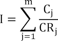
Where:
C j = Concentration of hazardous substance j in sample (or highest concentration of hazardous substance j from among comparable samples).
CR j = Screening concentration for noncancer toxicological responses corresponding to RfD or RfC for applicable exposure (inhalation or oral) for hazardous substance j.
m = Number of applicable hazardous substances in sample (or comparable samples) for which a CR j is available.
If either I or J equals or exceeds 1, consider the sampling location to be subject to Level I concentrations for that pathway (component or threat). If both I and J are less than 1, consider the sampling location to be subject to Level II concentrations for that pathway (component or threat). If, for the sampling location, there are sets of samples that are not comparable, calculate I and J separately for each such set, and use the highest calculated values of I and J to assign Level I and Level II.
See sections 7.3.1 and 7.3.2 for criteria for determining the level of contamination for radioactive substances.
3.0 Ground Water Migration Pathway
Evaluate the ground water migration pathway based on three factor categories: likelihood of release, waste characteristics, and targets. Figure 3-1 indicates the factors included within each factor category.
Determine the ground water migration pathway score (S gw) in terms of the factor category values as follows:
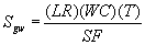
where:
LR = Likelihood of release factor category value.
WC = Waste characteristics factor category value.
T = Targets factor category value.
SF = Scaling factor.
Table 3-1 outlines the specific calculation procedure.
Calculate a separate ground water migration pathway score for each aquifer, using the factor category values for that aquifer for likelihood of release, waste characteristics, and targets. In doing so, include both the targets using water from that aquifer and the targets using water from all overlying aquifers through which the hazardous substances would migrate to reach the aquifer being evaluated. Assign the highest ground water migration pathway score that results for any aquifer as the ground water migration pathway score for the site.
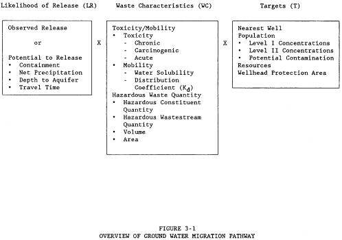
| Factor categories and factors | Maximum value | Value assigned |
| Likelihood of Release to an Aquifer: | ||
| 1. Observed Release | 550 | ___ |
| 2. Potential to Release: | ||
| 2a. Containment | 10 | ___ |
| 2b. Net Precipitation | 10 | ___ |
| 2c. Depth to Aquifer | 5 | ___ |
| 2d. Travel Time | 35 | ___ |
| 2e. Potential to Release [lines 2a(2b+2c+2d)] | 500 | ___ |
| 3. Likelihood of Release (higher of lines 1 and 2e) | 550 | ___ |
| Waste Characteristics: | ||
| 4. Toxicity/Mobility | (a) | ___ |
| 5. Hazardous Waste Quantity | (a) | ___ |
| 6. Waste Characteristics | 100 | ___ |
| Targets: | ||
| 7. Nearest Well | 50 | ___ |
| 8. Population: | ||
| 8a. Level I Concentrations | (b) | ___ |
| 8b. Level II Concentrations | (b) | ___ |
| 8c. Potential Contamination | (b) | ___ |
| 8d. Population (lines 8a+8b+8c) | (b) | ___ |
| 9. Resources | 5 | ___ |
| 10. Wellhead Protection Area | 20 | ___ |
| 11. Targets (lines 7+8d+9+10) | (b) | ___ |
| Ground Water Migration Score for an Aquifer: | ||
| 12. Aquifer Score [(lines 3x6x11)/82,500]c | 100 | ___ |
| Ground Water Migration Pathway Score: | ||
| 13. Pathway Score (Sgw), (highest value from line 12 for all aquifers evaluated)c | 100 | ___ |
a Maximum value applies to waste characteristics category.
b Maximum value not applicable.
c Do not round to nearest integer.
3.0.1 General considerations
3.0.1.1 Ground water target distance limit. The target distance limit defines the maximum distance from the sources at the site over which targets are evaluated. Use a target distance limit of 4 miles for the ground water migration pathway, except when aquifer discontinuities apply (see section 3.0.1.2.2). Furthermore, consider any well with an observed release from a source at the site (see section 3.1.1) to lie within the target distance limit of the site, regardless of the well's distance from the sources at the site.
For sites that consist solely of a contaminated ground water plume with no identified source, begin measuring the 4-mile target distance limit at the center of the area of observed ground water contamination. Determine the area of observed ground water contamination based on available samples that meet the criteria for an observed release.
3.0.1.2 Aquifer boundaries. Combine multiple aquifers into a single hydrologic unit for scoring purposes if aquifer interconnections can be established for these aquifers. In contrast, restrict aquifer boundaries if aquifer discontinuities can be established.
3.0.1.2.1 Aquifer interconnections. Evaluate whether aquifer interconnections occur within 2 miles of the sources at the site. If they occur within this 2-mile distance, combine the aquifers having interconnections in scoring the site. In addition, if observed ground water contamination attributable to the sources at the site extends beyond 2 miles from the sources, use any locations within the limits of this observed ground water contamination in evaluating aquifer interconnections. If data are not adequate to establish aquifer interconnections, evaluate the aquifers as separate aquifers.
3.0.1.2.2 Aquifer discontinuities. Evaluate whether aquifer discontinuities occur within the 4-mile target distance limit. An aquifer discontinuity occurs for scoring purposes only when a geologic, topographic, or other structure or feature entirely transects an aquifer within the 4-mile target distance limit, thereby creating a continuous boundary to ground water flow within this limit. If two or more aquifers can be combined into a single hydrologic unit for scoring purposes, an aquifer discontinuity occurs only when the structure or feature entirely transects the boundaries of this single hydrologic unit.
When an aquifer discontinuity is established within the 4-mile target distance limit, exclude that portion of the aquifer beyond the discontinuity in evaluating the ground water migration pathway. However, if hazardous substances have migrated across an apparent discontinuity within the 4-mile target distance limit, do not consider this to be a discontinuity in scoring the site.
3.0.1.3 Karst aquifer. Give a karst aquifer that underlies any portion of the sources at the site special consideration in the evaluation of two potential to release factors (depth to aquifer in section 3.1.2.3 and travel time in section 3.1.2.4), one waste characteristics factor (mobility in section 3.2.1.2), and two targets factors (nearest well in section 3.3.1 and potential contamination in section 3.3.2.4).
3.1 Likelihood of release. For an aquifer, evaluate the likelihood of release factor category in terms of an observed release factor or a potential to release factor.
3.1.1 Observed release. Establish an observed release to an aquifer by demonstrating that the site has released a hazardous substance to the aquifer. Base this demonstration on either:
- Direct observation—a material that contains one or more hazardous substances has been deposited into or has been observed entering the aquifer.
- Chemical analysis—an analysis of ground water samples from the aquifer indicates that the concentration of hazardous substance(s) has increased significantly above the background concentration for the site (see section 2.3). Some portion of the significant increase must be attributable to the site to establish the observed release, except: when the source itself consists of a ground water plume with no identified source, no separate attribution is required.
If an observed release can be established for the aquifer, assign the aquifer an observed release factor value of 550, enter this value in Table 3-1, and proceed to section 3.1.3. If an observed release cannot be established for the aquifer, assign an observed release factor value of 0, enter this value in Table 3-1, and proceed to section 3.1.2.
3.1.2 Potential to release. Evaluate potential to release only if an observed release cannot be established for the aquifer. Evaluate potential to release based on four factors: containment, net precipitation, depth to aquifer, and travel time. For sources overlying karst terrain, give any karst aquifer that underlies any portion of the sources at the site special consideration in evaluating depth to aquifer and travel time, as specified in sections 3.1.2.3 and 3.1.2.4.
3.1.2.1 Containment. Assign a containment factor value from Table 3-2 to each source at the site. Select the highest containment factor value assigned to those sources with a source hazardous waste quantity value of 0.5 or more (see section 2.4.2.1.5). (Do not include this minimum size requirement in evaluating any other factor of this pathway.) Assign this highest value as the containment factor value for the aquifer being evaluated. Enter this value in Table 3-1.
If no source at the site meets the minimum size requirement, then select the highest value assigned to the sources at the site and assign it as the containment factor value for the aquifer being evaluated. Enter this value in Table 3-1.
3.1.2.2 Net precipitation. Assign a net precipitation factor value to the site. Figure 3-2 provides computed net precipitation factor values, based on site location. Where necessary, determine the net precipitation factor value as follows:
- Determine monthly precipitation and monthly evapotranspiration:
- Use local measured monthly averages.
- When local data are not available, use monthly averages from the nearest National Oceanographic and Atmospheric Administration weather station that is in a similar geographic setting.
| Source | Assigned value |
| All Sources (Except Surface Impoundments, Land Treatment, Containers, and Tanks) | |
| Evidence of hazardous substance migration from source area (i.e. , source area includes source and any associated containment structures) | 10 |
| No liner | 10 |
| No evidence of hazardous substance migration from source area, a liner and: | |
| (a) None of the following present: (1) maintained engineered cover, or (2) functioning and maintained run-on control system and runoff management system, or (3) functioning leachate collection and removal system immediately above liner | 10 |
| (b) Any one of the three items in (a) present | 9 |
| (c) Any two of the items in (a) present | 7 |
| (d) All three items in (a) present plus a functioning ground water monitoring system | 5 |
| (e) All items in (d) present, plus no bulk or non-containerized liquids nor materials containing free liquids deposited in source area | 3 |
| No evidence of hazardous substance migration from source area, double liner with functioning leachate collection and removal system above and between liners, functioning ground water monitoring system, and: | |
| (f) Only one of the following deficiencies present in containment: (1) bulk or noncontainerized liquids or materials containing free liquids deposited in source area, or (2) no or nonfunctioning or nonmaintained run-on control system and runoff management system, or (3) no or nonmaintained engineered cover | 3 |
| (g) None of the deficiencies in (f) present | 0 |
| Source area inside or under maintained intact structure that provides protection from precipitation so that neither runoff nor leachate is generated, liquids or materials containing free liquids not deposited in source area, and functioning and maintained run-on control present | 0 |
| Surface Impoundment | |
| Evidence of hazardous substance migration from surface impoundment | 10 |
| No liner | 10 |
| Free liquids present with either no diking, unsound diking, or diking that is not regularly inspected and maintained | 10 |
| No evidence of hazardous substance migration from surface impoundment, free liquids present, sound diking that is regularly inspected and maintained, adequate freeboard, and: | |
| (a) Liner | 9 |
| (b) Liner with functioning leachate collection and removal system below liner, and functioning ground water monitoring system | 5 |
| (c) Double liner with functioning leachate collection and removal system between liners, and functioning ground water monitoring system | 3 |
| No evidence of hazardous substance migration from surface impoundment and all free liquids eliminated at closure (either by removal of liquids or solidification of remaining wastes and waste residues) | Evaluate using All sources criteria (with no bulk or free liquid deposited). |
| Land Treatment | |
| Evidence of hazardous substance migration from land treatment zone | 10 |
| No functioning, maintained, run-on control and runoff management system | 10 |
| No evidence of hazardous substance migration from land treatment zone and: | |
| (a) Functioning and maintained run-on control and runoff management system | 7 |
| (b) Functioning and maintained run-on control and runoff management system, and vegetative cover established over entire land treatment area | 5 |
| (c) Land treatment area maintained in compliance with 40 CFR 264.280 | 0 |
| Containers | |
| All containers buried | Evaluate using All sources criteria |
| Evidence of hazardous substance migration from container area (i.e., container area includes containers and any associated containment structures) | 10 |
| No liner (or no essentially impervious base) under container area. | 10 |
| No diking (or no similar structure) surrounding container area | 10 |
| Diking surrounding container area unsound or not regularly inspected and maintained | 10 |
| No evidence of hazardous substance migration from container area, container area surrounded by sound diking that is regularly inspected and maintained, and: | |
| (a) Liner (or essentially impervious base) under container area | 9 |
| (b) Essentially impervious base under container area with liquids collection and removal system | 7 |
| (c) Containment system includes essentially impervious base, liquids collection system, sufficient capacity to contain 10 percent of volume of all containers, and functioning and maintained run-on control; plus functioning ground water monitoring system, and spilled or leaked hazardous substances and accumulated precipitation removed in timely manner to prevent overflow of collection system, at least weekly inspection of containers, hazardous substances in leaking or deteriorating containers transferred to containers in good condition, and containers sealed except when waste is added or removed | 5 |
| (d) Free liquids present, containment system has sufficient capacity to hold total volume of all containers and to provide adequate freeboard, single liner under container area with functioning leachate collection and removal system below liner, and functioning ground water monitoring system | 5 |
| (e) Same as (d) except: double liner under container area with functioning leachate collection and removal system between liners | 3 |
| Containers inside or under maintained intact structure that provides protection from precipitation so that neither runoff nor leachate would be generated from any unsealed or ruptured containers, liquids or materials containing free liquids not deposited in any container, and functioning and maintained run-off control present | 0 |
| No evidence of hazardous substance migration from container area, containers leaking, and all free liquids eliminated at closure (either by removal of liquid or solidification of remaining wastes and waste residues) | Evaluate using All sources criteria (with no bulk or free liquid deposited). |
| Tank | |
| Below-ground tank | Evaluate using All sources criteria |
| Evidence of hazardous substance migration from tank area (i.e. , tank area includes tank, ancillary equipment such as piping, and any associated containment structures) | 10 |
| Tank and ancillary equipment not provided with secondary containment (e.g., liner under tank area, vault system, double wall) | 10 |
| No diking (or no similar structure) surrounding tank and ancillary equipment | 10 |
| Diking surrounding tank and ancillary equipment unsound or not regularly inspected and maintained | 10 |
| No evidence of hazardous substance migration from tank area, tank and ancillary equipment surrounded by sound diking that is regularly inspected and maintained, and: | |
| (a) Tank and ancillary equipment provided with secondary containment | 9 |
| (b) Tank and ancillary equipment provided with secondary containment with leak detection and collection system | 7 |
| (c) Tank and ancillary equipment provided with secondary containment system that detects and collects spilled or leaked hazardous substances and accumulated precipitation and has sufficient capacity to contain 110 percent of volume of largest tank within containment area, spilled or leaked hazardous substances and accumulated precipitation removed in timely manner, at least weekly inspection of tank and secondary containment system, all leaking or unfit-for-use tank systems promptly responded to, and functioning ground water monitoring system | 5 |
| (d) Containment system has sufficient capacity to hold volume of all tanks within tank containment area and to provide adequate freeboard, single liner under that containment area with functioning leachate collection and removal system below liner, and functioning ground water monitoring system | 5 |
| (e) Same as (d) except: double liner under tank containment area with functioning leachate collection and removal system between liners | 3 |
| Tank is above ground, and inside or under maintained intact structure that provides protection from precipitation so that neither runoff nor leachate would be generated from any material released from tank, liquids or materials containing free liquids not deposited in any tank, and functioning and maintained run-on control present | 0 |
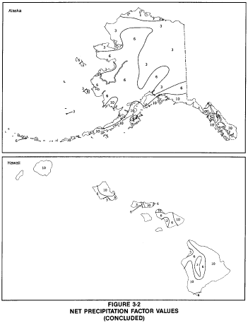
-When measured monthly evapotranspiration is not available, calculate monthly potential evapotranspiration (Ei) as follows:
E i = 0.6 F i (10 T i /I) a
where:
E i = Monthly potential evapotranspiration (inches) for month i.
F i = Monthly latitude adjusting value for month i.
T i = Mean monthly temperature (°C) for month i.
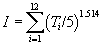
a = 6.75 × 10 -7 I 3 -7.71 × 10 -5 I 2 +
1.79 × 10 -2 I+0.49239
Select the latitude adjusting value for each month from Table 3-3. For latitudes lower than 50° North or 20° South, determine the monthly latitude adjusting value by interpolation.
- Calculate monthly net precipitation by subtracting monthly evapotranspiration (or monthly potential evapotranspiration) from monthly precipitation. If evapotranspiration (or potential evapotranspiration) exceeds precipitation for a month, assign that month a net precipitation value of 0.
- Calculate the annual net precipitation by summing the monthly net precipitation values.
- Based on the annual net precipitation, assign a net precipitation factor value from Table 3-4.
Enter the value assigned from Figure 3-2 or from Table 3-4, as appropriate, in Table 3-1.
| Latitude b (degrees) | Month | |||||||||||
| Jan. | Feb. | March | April | May | June | July | August | Sept. | Oct. | Nov. | Dec. | |
| ≥50 N | 0.74 | 0.78 | 1.02 | 1.15 | 1.33 | 1.36 | 1.37 | 1.25 | 1.06 | 0.92 | 0.76 | 0.70 |
| 45 N | 0.80 | 0.81 | 1.02 | 1.13 | 1.28 | 1.29 | 1.31 | 1.21 | 1.04 | 0.94 | 0.79 | 0.75 |
| 40 N | 0.84 | 0.83 | 1.03 | 1.11 | 1.24 | 1.25 | 1.27 | 1.18 | 1.04 | 0.96 | 0.83 | 0.81 |
| 35 N | 0.87 | 0.85 | 1.03 | 1.09 | 1.21 | 1.21 | 1.23 | 1.16 | 1.03 | 0.97 | 0.89 | 0.85 |
| 30 N | 0.90 | 0.87 | 1.03 | 1.08 | 1.18 | 1.17 | 1.20 | 1.14 | 1.03 | 0.98 | 0.89 | 0.88 |
| 20 N | 0.95 | 0.90 | 1.03 | 1.05 | 1.13 | 1.11 | 1.14 | 1.11 | 1.02 | 1.00 | 0.93 | 0.94 |
| 10 N | 1.00 | 0.91 | 1.03 | 1.03 | 1.08 | 1.06 | 1.08 | 1.07 | 1.02 | 1.02 | 0.98 | 0.99 |
| 0 | 1.04 | 0.94 | 1.04 | 1.01 | 1.04 | 1.01 | 1.04 | 1.04 | 1.01 | 1.04 | 1.01 | 1.04 |
| 10 S | 1.08 | 0.97 | 1.05 | 0.99 | 1.00 | 0.96 | 1.00 | 1.02 | 1.00 | 1.06 | 1.05 | 1.09 |
| 20 S | 1.14 | 0.99 | 1.05 | 0.97 | 0.96 | 0.91 | 0.95 | 0.99 | 1.00 | 1.08 | 1.09 | 1.15 |
a Do not round to nearest integer.
b For unlisted latitudes lower than 50° North or 20° South, determine the latitude adjusting value by interpolation.
| Net precipitation (inches) | Assigned value |
| 0 | 0 |
| Greater than 0 to 5 | 1 |
| Greater than 5 to 15 | 3 |
| Greater than 15 to 30 | 6 |
| Greater than 30 | 10 |
3.1.2.3 Depth to aquifer. Evaluate depth to aquifer by determining the depth from the lowest known point of hazardous substances at a site to the top of the aquifer being evaluated, considering all layers in that interval. Measure the depth to an aquifer as the distance from the surface to the top of the aquifer minus the distance from the surface to the lowest known point of hazardous substances eligible to be evaluated for that aquifer. In evaluating depth to aquifer in karst terrain, assign a thickness of 0 feet to a karst aquifer that underlies any portion of the sources at the site. Based on the calculated depth, assign a value from Table 3-5 to the depth to aquifer factor.
Determine the depth to aquifer only at locations within 2 miles of the sources at the site, except: if observed ground water contamination attributable to sources at the site extends more than 2 miles beyond these sources, use any location within the limits of this observed ground water contamination when evaluating the depth to aquifer factor for any aquifer that does not have an observed release. If the necessary geologic information is available at multiple locations, calculate the depth to aquifer at each location. Use the location having the smallest depth to assign the factor value. Enter this value in Table 3-1.
| Depth to aquifera (feet) | Assigned value |
| Less than or equal to 25 | 5 |
| Greater than 25 to 250 | 3 |
| Greater than 250 | 1 |
a Use depth of all layers between the hazardous substances and aquifer. Assign a thickness of 0 feet to any karst aquifer that underlies any portion of the sources at the site.
3.1.2.4 Travel time. Evaluate the travel time factor based on the geologic materials in the interval between the lowest known point of hazardous substances at the site and the top of the aquifer being evaluated. Assign a value to the travel time factor as follows:
- If the depth to aquifer (see section 3.1.2.3) is 10 feet or less, assign a value of 35.
- If, for the interval being evaluated, all layers that underlie a portion of the sources at the site are karst, assign a value of 35.
- Otherwise:
- Select the lowest hydraulic conductivity layer(s) from within the above interval. Consider only layers at least 3 feet thick. However, do not consider layers or portions of layers within the first 10 feet of the depth to the aquifer.
- Determine hydraulic conductivities for individual layers from Table 3-6 or from in-situ or laboratory tests. Use representative, measured, hydraulic conductivity values whenever available.
- If more than one layer has the same lowest hydraulic conductivity, include all such layers and sum their thicknesses. Assign a thickness of 0 feet to a karst layer that underlies any portion of the sources at the site.
- Assign a value from Table 3-7 to the travel time factor, based on the thickness and hydraulic conductivity of the lowest hydraulic conductivity layer(s).
| Type of material | Assigned hydraulic conductivitya (cm/sec) |
| Clay; low permeability till (compact unfractured till); shale; unfractured metamorphic and igneous rocks | 10−8 |
| Silt; loesses; silty clays; sediments that are predominantly silts; moderately permeable till (fine-grained, unconsolidated till, or compact till with some fractures); low permeability limestones and dolomites (no karst); low permeability sandstone; low permeability fractured igneous and metamorphic rocks | 10−6 |
| Sands; sandy silts; sediments that are predominantly sand; highly permeable till (coarse-grained, unconsolidated or compact and highly fractured); peat; moderately permeable limestones and dolomites (no karst); moderately permeable sandstone; moderately permeable fractured igneous and metamorphic rocks | 10−4 |
| Gravel; clean sand; highly permeable fractured igneous and metamorphic rocks; permeable basalt; karst limestones and dolomites | 10−2 |
a Do not round to nearest integer.
| Hydraulic conductivity (cm/sec) | Thickness of lowest hydraulic conductivity layer(s)b (feet) | |||
| Greater than 3 to 5 | Greater than 5 to 100 | Greater than 100 to 500 | Greater than 500 | |
| Greater than or equal to 10−3 | 35 | 35 | 35 | 25 |
| Less than 10−3 to 10−5 | 35 | 25 | 15 | 15 |
| Less than 10 −5 to 10−7 | 15 | 15 | 5 | 5 |
| Less than 10−7 | 5 | 5 | 1 | 1 |
a If depth to aquifer is 10 feet or less or if, for the interval being evaluated, all layers that underlie a portion of the sources at the site are karst, assign a value of 35.
b Consider only layers at least 3 feet thick. Do not consider layers or portions of layers within the first 10 feet of the depth to the aquifer.
Determine travel time only at locations within 2 miles of the sources at the site, except: if observed ground water contamination attributable to sources at the site extends more than 2 miles beyond these sources, use any location within the limits of this observed ground water contamination when evaluating the travel time factor for any aquifer that does not have an observed release. If the necessary subsurface geologic information is available at multiple locations, evaluate the travel time factor at each location. Use the location having the highest travel time factor value to assign the factor value for the aquifer. Enter this value in Table 3-1.
3.1.2.5 Calculation of potential to release factor value. Sum the factor values for net precipitation, depth to aquifer, and travel time, and multiply this sum by the factor value for containment. Assign this product as the potential to release factor value for the aquifer. Enter this value in Table 3-1.
3.1.3 Calculation of likelihood of release factor category value. If an observed release is established for an aquifer, assign the observed release factor value of 550 as the likelihood of release factor category value for that aquifer. Otherwise, assign the potential to release factor value for that aquifer as the likelihood of release value. Enter the value assigned in Table 3-1.
3.2 Waste characteristics. Evaluate the waste characteristics factor category for an aquifer based on two factors: toxicity/mobility and hazardous waste quantity. Evaluate only those hazardous substances available to migrate from the sources at the site to ground water. Such hazardous substances include:
- Hazardous substances that meet the criteria for an observed release to ground water.
- All hazardous substances associated with a source that has a ground water containment factor value greater than 0 (see sections 2.2.2, 2.2.3, and 3.1.2.1).
3.2.1 Toxicity/mobility. For each hazardous substance, assign a toxicity factor value, a mobility factor value, and a combined toxicity/mobility factor value as specified in the following sections. Select the toxicity/ mobility factor value for the aquifer being evaluated as specified in section 3.2.1.3.
3.2.1.1 Toxicity. Assign a toxicity factor value to each hazardous substance as specified in Section 2.4.1.1.
3.2.1.2 Mobility. Assign a mobility factor value to each hazardous substance for the aquifer being evaluated as follows:
- For any hazardous substance that meets the criteria for an observed release by chemical analysis to one or more aquifers underlying the sources at the site, regardless of the aquifer being evaluated, assign a mobility factor value of 1.
- For any hazardous substance that does not meet the criteria for an observed release by chemical analysis to at least one of the aquifers, assign that hazardous substance a mobility factor value from Table 3-8 for the aquifer being evaluated, based on its water solubility and distribution coefficient (Kd).
- If the hazardous substance cannot be assigned a mobility factor value because data on its water solubility or distribution coefficient are not available, use other hazardous substances for which information is available in evaluating the pathway.
| Water solubility (mg/l) | Distribution coefficient (Kd) (ml/g) | |||
| Karstc | ≤10 | >10 to 1,000 | >1,000 | |
| Present as liquidb | 1 | 1 | 0.01 | 0.0001 |
| Greater than 100 | 1 | 1 | 0.01 | 0.0001 |
| Greater than 1 to 100 | 0.2 | 0.2 | 0.002 | 2×10⁻⁵ |
| Greater than 0.01 to 1 | 0.002 | 0.002 | 2×10 −5 | 2×10 −7 |
| Less than or equal to 0.01 | 2×10 −5 | 2×10 −5 | 2×10 −7 | 2×10 −9 |
a Do not round to nearest integer.
b Use if the hazardous substance is present or deposited as a liquid.
c Use if the entire interval from the source to the aquifer being evaluated is karst.
- If none of the hazardous substances eligible to be evaluated can be assigned a mobility factor value, use a default value of 0.002 as the mobility factor value for all these hazardous substances.
Determine the water solubility to be used in Table 3-8 for the hazardous substance as follows (use this same water solubility for all aquifers):
- For any hazardous substance that does not meet the criteria for an observed release by chemical analysis, if the hazardous substance is present or deposited as a liquid, use the water solubility category "Present as Liquid" in Table 3-8 to assign the mobility factor value to that hazardous substance.
-
Otherwise:
-
For any hazardous substance that is a metal (or metalloid) and that does not meet the criteria for an observed release by chemical analysis, establish a water solubility for the hazardous substance as follows:
- Determine the overall range of water solubilities for compounds of this hazardous substance (consider all compounds for which adequate water solubility information is available, not just compounds identified as present at the site).
- Calculate the geometric mean of the highest and the lowest water solubility in this range.
- Use this geometric mean as the water solubility in assigning the hazardous substance a mobility factor value from Table 3-8.
- For any other hazardous substance (either organic or inorganic) that does not meet the criteria for an observed release by chemical analysis, use the water solubility of that hazardous substance to assign a mobility factor value from Table 3-8 to the hazardous substance.
-
For any hazardous substance that is a metal (or metalloid) and that does not meet the criteria for an observed release by chemical analysis, establish a water solubility for the hazardous substance as follows:
For the aquifer being evaluated, determine the distribution coefficient to be used in Table 3-8 for the hazardous substance as follows:
- For any hazardous substance that does not meet the criteria for an observed release by chemical analysis, if the entire interval from a source at the site to the aquifer being evaluated is karst, use the distribution coefficient category "Karst" in Table 3-8 in assigning the mobility factor value for that hazardous substance for that aquifer.
-
Otherwise:
- For any hazardous substance that is a metal (or metalloid) and that does not meet the criteria for an observed release by chemical analysis, use the distribution coefficient for the metal or (metalloid) to assign a mobility factor value from Table 3-8 for that hazardous substance.
- For any other inorganic hazardous substance that does not meet the criteria for an observed release by chemical analysis, use the distribution coefficient for that inorganic hazardous substance, if available, to assign a mobility factor value from Table 3-8. If the distribution coefficient is not available, use a default value of "less than 10" as the distribution coefficient, except: for asbestos use a default value of "greater than 1,000" as the distribution coefficient.
-
For any hazardous substance that is organic and that does not meet the criteria for an observed release by chemical analysis, establish a distribution coefficient for that hazardous substance as follows:
- Estimate the K d range for the hazardous substance using the following equation:
K d = (K oc)(f s)
where:
K oc = Soil-water partition coefficient for organic carbon for the hazardous substance.
f s = Sorbent content (fraction of clays plus organic carbon) in the subsurface.
- Use f s values of 0.03 and 0.77 in the above equation to establish the upper and lower values of the K d range for the hazardous substance.
- Calculate the geometric mean of the upper and lower K d range values. Use this geometric mean as the distribution coefficient in assigning the hazardous substance a mobility factor value from Table 3-8.
3.2.1.3 Calculation of toxicity/mobility factor value. Assign each hazardous substance a toxicity/mobility factor value from Table 3-9, based on the values assigned to the hazardous substance for the toxicity and mobility factors. Use the hazardous substance with the highest toxicity/mobility factor value for the aquifer being evaluated to assign the value to the toxicity/mobility factor for that aquifer. Enter this value in Table 3-1.
| Mobility factor value | Toxicity factor value | |||||
| 10,000 | 1,000 | 100 | 10 | 1 | 0 | |
| 1.0 | 10,000 | 1,000 | 100 | 10 | 1 | 0 |
| 0.2 | 2,000 | 200 | 20 | 2 | 0.2 | 0 |
| 0.01 | 100 | 10 | 1 | 0.1 | 0.01 | 0 |
| 0.002 | 20 | 2 | 0.2 | 0.02 | 0.002 | 0 |
| 0.0001 | 1 | 0.1 | 0.01 | 0.001 | 1×10 −4 | 0 |
| 2×10 −5 | 0.2 | 0.02 | 0.002 | 2×10 −4 | 2×10 −5 | 0 |
| 2×10 −7 | 0.002 | 2×10 −4 | 2×10 −5 | 2×10 −6 | 2×10 −7 | 0 |
| 2×10 −9 | 2×10 −5 | 2×10 −6 | 2×10 −7 | 2×10 −8 | 2×10 −9 | 0 |
a Do not round to nearest integer.
3.2.2 Hazardous waste quantity. Assign a hazardous waste quantity factor value for the ground water pathway (or aquifer) as specified in section 2.4.2. Enter this value in Table 3-1.
3.2.3 Calculation of waste characteristics factor category value. Multiply the toxicity/mobility and hazardous waste quantity factor values, subject to a maximum product of 1x10 8. Based on this product, assign a value from Table 2-7 (section 2.4.3.1) to the waste characteristics factor category. Enter this value in Table 3-1.
3.3 Targets. Evaluate the targets factor category for an aquifer based on four factors: nearest well, population, resources, and Wellhead Protection Area. Evaluate these four factors based on targets within the target distance limit specified in section 3.0.1.1 and the aquifer boundaries specified in section 3.0.1.2. Determine the targets to be included in evaluating these factors for an aquifer as specified in section 3.0.
3.3.1 Nearest well. In evaluating the nearest well factor, include both the drinking water wells drawing from the aquifer being evaluated and those drawing from overlying aquifers as specified in section 3.0. Include standby wells in evaluating this factor only if they are used for drinking water supply at least once every year.
If there is an observed release by direct observation for a drinking water well within the target distance limit, assign Level II concentrations to that well. However, if one or more samples meet the criteria for an observed release for that well, determine if that well is subject to Level I or Level II concentrations as specified in sections 2.5.1 and 2.5.2. Use the health- based benchmarks from Table 3-10 in determining the level of contamination.
Assign a value for the nearest well factor as follows:
- If one or more drinking water wells is subject to Level I concentrations, assign a value of 50.
- If not, but if one or more drinking water wells is subject to Level II concentrations, assign a value of 45.
-
If none of the drinking water wells is subject to Level I or Level II concentrations, assign a value as follows:
- If one of the target aquifers is a karst aquifer that underlies any portion of the sources at the site and any well draws drinking water from this karst aquifer within the target distance limit, assign a value of 20.
- If not, determine the shortest distance to any drinking water well, as measured from any source at the site with a ground water containment factor value greater than 0. Select a value from Table 3-11 based on this distance. Assign it as the value for the nearest well factor.
Enter the value assigned to the nearest well factor in Table 3-1.
| • Concentration corresponding to Maximum Contaminant Level (MCL). |
| • Concentration corresponding to a nonzero Maximum Contaminant Level Goal (MCLG). |
| • Screening concentration for cancer corresponding to that concentration that corresponds to the 10 −6 individual cancer risk for oral exposures. |
| • Screening concentration for noncancer toxicological responses corresponding to the Reference Dose (RfD) for oral exposures. |
| Distance from source (miles) | Assigned value |
| Level I concentrations a | 50 |
| Level II concentrations a | 45 |
| 0 to 1/4 | 20 |
| Greater than 1/4 to 1/2 | 18 |
| Greater than 1/2 to 1 | 9 |
| Greater than 1 to 2 | 5 |
| Greater than 2 to 3 | 3 |
| Greater than 3 to 4 | 2 |
| Greater than 4 | 0 |
a Distance does not apply.
3.3.2 Population. In evaluating the population factor, include those persons served by drinking water wells within the target distance limit specified in section 3.0.1.1. For the aquifer being evaluated, count those persons served by wells in that aquifer and those persons served by wells in overlying aquifers as specified in section 3.0. Include residents, students, and workers who regularly use the water. Exclude transient populations such as customers and travelers passing through the area. Evaluate the population based on the location of the water supply wells, not on the location of residences, work places, etc. When a standby well is maintained on a regular basis so that water can be withdrawn, include it in evaluating the population factor.
In estimating residential population, when the estimate is based on the number of residences, multiply each residence by the average number of persons per residence for the county in which the residence is located.
In determining the population served by a well, if the water from the well is blended with other water (for example, water from other ground water wells or surface water intakes), apportion the total population regularly served by the blended system to the well based on the well's relative contribution to the total blended system. In estimating the well's relative contribution, assume each well and intake contributes equally and apportion the population accordingly, except: if the relative contribution of any one well or intake exceeds 40 percent based on average annual pumpage or capacity, estimate the relative contribution of the wells and intakes considering the following data, if available:
- Average annual pumpage from the ground water wells and surface water intakes in the blended system.
- Capacities of the wells and intakes in the blended system.
For systems with standby ground water wells or standby surface water intakes, apportion the total population regularly served by the blended system as described above, except:
- Exclude standby surface water intakes in apportioning the population.
- When using pumpage data for a standby ground water well, use average pumpage for the period during which the standby well is used rather than average annual pumpage.
- For that portion of the total population that could be apportioned to a standby ground water well, assign that portion of the population either to that standby well or to the other ground water well(s) and surface water intake(s) that serve that population; do not assign that portion of the population both to the standby well and to the other well(s) and intake(s) in the blended system. Use the apportioning that results in the highest population factor value. (Either include all standby well(s) or exclude some or all of the standby well(s) as appropriate to obtain this highest value.) Note that the specific standby well(s) included or excluded and, thus, the specific apportioning may vary in evaluating different aquifers and in evaluating the surface water pathway.
3.3.2.1 Level of contamination. Evaluate the population served by water from a point of withdrawal based on the level of contamination for that point of withdrawal. Use the applicable factor: Level I concentrations, Level II concentrations, or potential contamination.
If no samples meet the criteria for an observed release for a point of withdrawal and there is no observed release by direct observation for that point of withdrawal, evaluate that point of withdrawal using the potential contamination factor in section 3.3.2.4. If there is an observed release by direct observation, use Level II concentrations for that point of withdrawal. However, if one or more samples meet the criteria for an observed release for the point of withdrawal, determine which factor (Level I or Level II concentrations) applies to that point of withdrawal as specified in sections 2.5.1 and 2.5.2. Use the health-based benchmarks from Table 3-10 in determining the level of contamination. Evaluate the point of withdrawal using the Level I concentrations factor in section 3.3.2.2 or the Level II concentrations factor in section 3.3.2.3, as appropriate.
For the potential contamination factor, use population ranges in evaluating the factor as specified in section 3.3.2.4. For the Level I and Level II concentrations factors, use the population estimate, not population ranges, in evaluating both factors.
3.3.2.2 Level I concentrations. Sum the number of people served by drinking water from points of withdrawal subject to Level I concentrations. Multiply this sum by 10. Assign this product as the value for this factor. Enter this value in Table 3-1.
3.3.2.3 Level II concentrations. Sum the number of people served by drinking water from points of withdrawal subject to Level II concentrations. Do not include those people already counted under the Level I concentrations factor. Assign this sum as the value for this factor. Enter this value in Table 3-1.
3.3.2.4 Potential contamination. Determine the number of people served by drinking water from points of withdrawal subject to potential contamination. Do not include those people already counted under the Level I and Level II concentrations factors.
Assign distance-weighted population values from Table 3-12 to this population as follows:
-
Use the "Karst" portion of Table 3-12 to assign values only for that portion of the population served by points of withdrawal that draw drinking water from a karst aquifer that underlies any portion of the sources at the site.
- For this portion of the population, determine the number of people included within each "Karst" distance category in Table 3-12.
| Distance category (miles) | Number of people within the distance category | ||||||||||||
| 0 | 1 to 10 | 11 to 30 | 31 to 100 | 101 to 300 | 301 to 1,000 | 1,001 to 3,000 | 3,001 to 10,000 | 10,001 to 30,000 | 30,001 to 100,000 | 100,001 to 300,000 | 300,001 to 1,000,000 | 1,000,001 to 3,000,000 | |
| Other Than Karst b: | |||||||||||||
| 0 to 1/4 | 0 | 4 | 17 | 53 | 164 | 522 | 1,633 | 5,214 | 16,325 | 52,137 | 163,246 | 521,360 | 1,632,455 |
| Greater than 1/4 to 1/2 | 0 | 2 | 11 | 33 | 102 | 324 | 1,013 | 3,233 | 10,122 | 32,325 | 101,213 | 323,243 | 1,012,122 |
| Greater than 1/2 to 1 | 0 | 1 | 5 | 17 | 52 | 167 | 523 | 1,669 | 5,224 | 16,684 | 52,239 | 166,835 | 522,385 |
| Greater than 1 to 2 | 0 | 0.7 | 3 | 10 | 30 | 94 | 294 | 939 | 2,939 | 9,385 | 29,384 | 93,845 | 293,842 |
| Greater than 2 to 3 | 0 | 0.5 | 2 | 7 | 21 | 68 | 212 | 678 | 2,122 | 6,778 | 21,222 | 67,777 | 212,219 |
| Greater than 3 to 4 | 0 | 0.3 | 1 | 4 | 13 | 42 | 131 | 417 | 1,306 | 4,171 | 13,060 | 41,709 | 130,596 |
| Karst c: | |||||||||||||
| 0 to 1/4 | 0 | 4 | 17 | 53 | 164 | 522 | 1,633 | 5,214 | 16,325 | 52,137 | 163,246 | 521,360 | 1,632,455 |
| Greater than 1/4 to 1/2 | 0 | 2 | 11 | 33 | 102 | 324 | 1,013 | 3,233 | 10,122 | 32,325 | 101,213 | 323,243 | 1,012,122 |
| Greater than 1/2 to 1 | 0 | 2 | 9 | 26 | 82 | 261 | 817 | 2,607 | 8,163 | 26,068 | 81,623 | 260,680 | 816,227 |
| Greater than 1 to 2 | 0 | 2 | 9 | 26 | 82 | 261 | 817 | 2,607 | 8,163 | 26,068 | 81,623 | 260,680 | 816,227 |
| Greater than 2 to 3 | 0 | 2 | 9 | 26 | 82 | 261 | 817 | 2,607 | 8,163 | 26,068 | 81,623 | 260,680 | 816,227 |
| Greater than 3 to 4 | 0 | 2 | 9 | 26 | 82 | 261 | 817 | 2,607 | 8,163 | 26,068 | 81,623 | 260,680 | 816,227 |
a Round the number of people present within a distance category to nearest integer. Do not round the assigned distance-weighted population value to nearest integer.
b Use for all aquifers, except karst aquifers underlying any portion of the sources at the site.
c Use only for karst aquifers underlying any portion of the sources at the site.
-Assign a distance-weighted population value for each distance category based on the number of people included within the distance category.
-
Use the "Other Than Karst" portion of Table 3-12 for the remainder of the population served by points of withdrawal subject to potential contamination.
- For this portion of the population, determine the number of people included within each "Other Than Karst" distance category in Table 3-12.
- Assign a distance-weighted population value for each distance category based on the number of people included within the distance category.
Calculate the value for the potential contamination factor (PC) as follows:
where:
W i = Distance-weighted population from "Other Than Karst" portion of Table 3-12 for distance category i.
K i = Distance-weighted population from "Karst" portion of Table 3-12 for distance category i.
n = Number of distance categories.
If PC is less than 1, do not round it to the nearest integer; if PC is 1 or more, round to the nearest integer. Enter this value in Table 3-1.
3.3.2.5 Calculation of population factor value. Sum the factor values for Level I concentrations, Level II concentrations, and potential contamination. Do not round this sum to the nearest integer. Assign this sum as the population factor value for the aquifer. Enter this value in Table 3-1.
3.3.3 Resources. To evaluate the resources factor, select the highest value specified below that applies for the aquifer being evaluated. Assign this value as the resources factor value for the aquifer. Enter this value in Table 3-1.
Assign a resources value of 5 if water drawn from any target well for the aquifer being evaluated or overlying aquifers (as specified in section 3.0) is used for one or more of the following purposes:
- Irrigation (5-acre minimum) of commercial food crops or commercial forage crops.
- Watering of commercial livestock.
- Ingredient in commercial food preparation.
- Supply for commercial aquaculture.
- Supply for a major or designated water recreation area, excluding drinking water use.
Assign a resources value of 5 if no drinking water wells are within the target distance limit, but the water in the aquifer being evaluated or any overlying aquifers (as specified in section 3.0) is usable for drinking water purposes.
Assign a resources value of 0 if none of the above applies.
3.3.4 Wellhead Protection Area. Evaluate the Wellhead Protection Area factor based on Wellhead Protection Areas designated according to section 1428 of the Safe Drinking Water Act, as amended. Consider only those Wellhead Protection Areas applicable to the aquifer being evaluated or overlying aquifers (as specified in section 3.0). Select the highest value below that applies. Assign it as the value for the Wellhead Protection Area factor for the aquifer being evaluated. Enter this value in Table 3-1.
Assign a value of 20 if either of the following criteria applies for the aquifer being evaluated or overlying aquifers:
- A source with a ground water containment factor value greater than 0 lies, either partially or fully, within or above the designated Wellhead Protection Area.
- Observed ground water contamination attributable to the sources at the site lies, either partially or fully, within the designated Wellhead Protection Area.
If neither criterion applies, assign a value of 5, if, within the target distance limit, there is a designated Wellhead Protection Area applicable to the aquifer being evaluated or overlying aquifers.
Assign a value of 0 if none of the above applies.
3.3.5 Calculation of targets factor category value. Sum the factor values for nearest well, population, resources, and Wellhead Protection Area. Do not round this sum to the nearest integer. Use this sum as the targets factor category value for the aquifer. Enter this value in Table 3-1.
3.4 Ground water migration score for an aquifer. For the aquifer being evaluated, multiply the factor category values for likelihood of release, waste characteristics, and targets, and round the product to the nearest integer. Then divide by 82,500. Assign the resulting value, subject to a maximum value of 100, as the ground water migration pathway score for the aquifer. Enter this score in Table 3-1.
3.5 Calculation of ground water migration pathway score. Calculate a ground water migration score for each aquifer underlying the sources at the site, as appropriate. Assign the highest ground water migration score for an aquifer as the ground water migration pathway score (S gw) for the site. Enter this score in Table 3-1.
4.0 Surface Water Migration Pathway.
4.0.1 Migration components. Evaluate the surface water migration pathway based on two migration components:
- Overland/flood migration to surface water (see section 4.1).
- Ground water to surface water migration (see section 4.2).
Evaluate each component based on the same three threats: drinking water threat, human food chain threat, and environmental threat.
Score one or both components, considering their relative importance. If only one component is scored, assign its score as the surface water migration pathway score. If both components are scored, select the higher of the two scores and assign it as the surface water migration pathway score.
4.0.2 Surface water categories. For HRS purposes, classify surface water into four categories: rivers, lakes, oceans, and coastal tidal waters.
Rivers include:
- Perennially flowing waters from point of origin to the ocean or to coastal tidal waters, whichever comes first, and wetlands contiguous to these flowing waters.
- Aboveground portions of disappearing rivers.
- Man-made ditches only insofar as they perennially flow into other surface water.
- Intermittently flowing waters and contiguous intermittently flowing ditches only in arid or semiarid areas with less than 20 inches of mean annual precipitation.
Lakes include:
- Natural and man-made lakes (including impoundments) that lie along rivers, but excluding the Great Lakes.
- Isolated, but perennial, lakes, ponds, and wetlands.
- Static water channels or oxbow lakes contiguous to rivers.
- Small rivers, without diking, that merge into surrounding perennially inundated wetlands.
- Wetlands contiguous to water bodies defined here as lakes.
Ocean and ocean-like water bodies include:
- Ocean areas seaward from the baseline of the Territorial Sea. (This baseline represents the generalized coastline of the United States. It is parallel to the seaward limit of the Territorial Sea and other maritime limits such as the inner boundary of Federal fisheries jurisdiction and the limit of States jurisdiction under the Submerged Lands Act, as amended.)
- The Great Lakes.
- Wetlands contiguous to the Great Lakes.
Coastal tidal waters include:
- Embayments, harbors, sounds, estuaries, back bays, lagoons, wetlands, etc. seaward from mouths of rivers and landward from the baseline of the Territorial Sea.
4.1 Overland/flood migration component. Use the overland/flood migration component to evaluate surface water threats that result from overland migration of hazardous substances from a source at the site to surface water. Evaluate three types of threats for this component: drinking water threat, human food chain threat, and environmental threat.
4.1.1 General considerations.
4.1.1.1 Definition of hazardous substance migration path for overland/ flood migration component. The hazardous substance migration path includes both the overland segment and the in-water segment that hazardous substances would take as they migrate away from sources at the site:
- Begin the overland segment at a source and proceed downgradient to the probable point of entry to surface water.
-
Begin the in-water segment at this probable point of entry.
- For rivers, continue the in-water segment in the direction of flow (including any tidal flows) for the distance established by the target distance limit (see section 4.1.1.2).
- For lakes, oceans, coastal tidal waters, or Great Lakes, do not consider flow direction. Instead apply the target distance limit as an arc.
- -If the in-water segment includes both rivers and lakes (or oceans, coastal tidal waters, or Great Lakes), apply the target distance limit to their combined in-water segments.
For sites that consist of contaminated sediments with no identified source, the hazardous substance migration path consists solely of the in-water segment specified in section 4.1.1.2.
Consider a site to be in two or more watersheds for this component if two or more hazardous substance migration paths from the sources at the site do not reach a common point within the target distance limit. If the site is in more than one watershed, define a separate hazardous substance migration path for each watershed. Evaluate the overland/flood migration component for each watershed separately as specified in section 4.1.1.3.
4.1.1.2 Target distance limit. The target distance limit defines the maximum distance over which targets are considered in evaluating the site. Determine a separate target distance limit for each watershed as follows:
- If there is no observed release to surface water in the watershed or if there is an observed release only by direct observation (see section 4.1.2.1.1), begin measuring the target distance limit for the watershed at the probable point of entry to surface water and extend it for 15 miles along the surface water from that point.
- If there is an observed release from the site to the surface water in the watershed that is based on sampling, begin measuring the target distance limit for the watershed at the probable point of entry; extend the target distance limit either for 15 miles along the surface water or to the most distant sample point that meets the criteria for an observed release to that watershed, whichever is greater.
In evaluating the site, include only surface water targets (for example, intakes, fisheries, sensitive environments) that are within or contiguous to the hazardous substance migration path and located, partially or wholly, at or between the probable point of entry and the target distance limit applicable to the watershed:
- If flow within the hazardous substance migration path is reversed by tides, evaluate upstream targets only if there is documentation that the tidal run could carry substances from the site as far as those upstream targets.
-
Determine whether targets within or contiguous to the hazardous substance migration path are subject to actual or potential contamination as follows:
- If a target is located, partially or wholly, either at or between the probable point of entry and any sampling point that meets the criteria for an observed release to the watershed or at a point that meets the criteria for an observed release by direct observation, evaluate that target as subject to actual contamination, except as otherwise specified for fisheries in section 4.1.3.3 and for wetlands in section 4.1.4.3.1.1. If the actual contamination is based on direct observation, assign Level II to the actual contamination. However, if the actual contamination is based on samples, determine whether the actual contamination is at Level I or Level II concentrations as specified in sections 4.1.2.3, 4.1.3.3, and 4.1.4.3.1.
- If a target is located, partially or wholly, within the target distance limit for the watershed, but not at or between the probable point of entry and any sampling point that meets the criteria for an observed release to the watershed, nor at a point that meets the criteria for an observed release by direct observation, evaluate it as subject to potential contamination.
For sites consisting solely of contaminated sediments with no identified source, determine the target distance limit as follows:
- If there is a clearly defined direction of flow for the surface water body (or bodies) containing the contaminated sediments, begin measuring the target distance limit at the point of observed sediment contamination that is farthest upstream (that is, at the location of the farthest available upstream sediment sample that meets the criteria for an observed release); extend the target distance limit either for 15 miles along the surface water or to the most distant downstream sample point that meets the criteria for an observed release to that watershed, whichever is greater.
- If there is no clearly defined direction of flow, begin measuring the target distance limit at the center of the area of observed sediment contamination. Extend the target distance limit as an arc either for 15 miles along the surface water or to the most distant sample point that meets the criteria for an observed release to that watershed, whichever is greater. Determine the area of observed sediment contamination based on available samples that meet the criteria for an observed release.
Note that the hazardous substance migration path for these contaminated sediment sites consists solely of the in-water segment defined by the target distance limit; there is no overland segment.
For these contaminated sediment sites, include only those targets (for example, intakes, fisheries, sensitive environments) that are within or contiguous to the hazardous substance migration path and located, wholly or partially, within the target distance limit for the site. Determine whether these targets are subject to actual or potential contamination as follows:
-
If a target is located, partially or wholly, within the area of observed sediment contamination, evaluate it as subject to actual contamination, except as otherwise specified for fisheries in section 4.1.3.3 and wetlands in section 4.1.4.3.1.1.
- If a drinking water target is subject to actual contamination, evaluate it using Level II concentrations.
- If a human food chain target or environmental target is subject to actual contamination, evaluate it using Level I or Level II concentrations, as appropriate (see sections 4.1.3.3 and 4.1.4.3.1).
- If a target is located, partially or wholly, within the target distance limit for the watershed, but not within the area of observed sediment contamination, evaluate it as subject to potential contamination.
4.1.1.3 Evaluation of overland/flood migration component. Evaluate the drinking water threat, human food chain threat, and environmental threat for each watershed for this component based on three factor categories: likelihood of release, waste characteristics, and targets. Figure 4-1 indicates the factors included within each factor category for each type of threat.
Determine the overland/flood migration component score (S of) for a watershed in terms of the factor category values as follows:
where:
LR i = Likelihood of release factor category value for threat i (that is, drinking water, human food chain, or environmental threat).
WC i = Waste characteristics factor category value for threat i.
T i = Targets factor category value for threat i.
SF = Scaling factor.
Table 4-1 outlines the specific calculation procedure.
If the site is in only one watershed, assign the overland/flood migration score for that watershed as the overland/flood migration component score for the site.
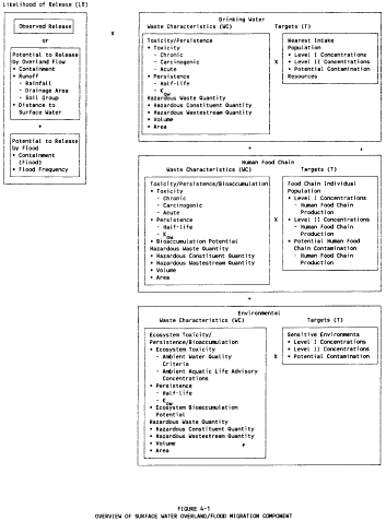
| Factor categories and factors | Maximum value | Value assigned |
| Drinking Water Threat | ||
| Likelihood of Release: | ||
| 1. Observed Release | 550 | ___ |
| 2. Potential to Release by Overland Flow: | ||
| 2a. Containment | 10 | ___ |
| 2b. Runoff | 25 | ___ |
| 2c. Distance to Surface Water | 25 | ___ |
| 2d. Potential to Release by Overland Flow (lines 2a[2b+2c]) | 500 | ___ |
| 3. Potential to Release by Flood: | ||
| 3a. Containment (Flood) | 10 | ___ |
| 3b. Flood Frequency | 50 | ___ |
| 3c. Potential to Release by Flood (lines 3a×3b) | 500 | ___ |
| 4. Potential to Release (lines 2d+3c, subject to a maximum of 500) | 500 | ___ |
| 5. Likelihood of Release (higher of lines 1 and 4) | 550 | ___ |
| Waste Characteristics: | ||
| 6. Toxicity/Persistence | (a) | ___ |
| 7. Hazardous Waste Quantity | (a) | ___ |
| 8. Waste Characteristics | 100 | ___ |
| Targets: | ||
| 9. Nearest Intake | 50 | ___ |
| 10. Population | ||
| 10a. Level I Concentrations | (b) | ___ |
| 10b. Level II Concentrations | (b) | ___ |
| 10c. Potential Contamination | (b) | ___ |
| 10d. Population (lines 10a+10b+10c) | (b) | ___ |
| 11. Resources | 5 | ___ |
| 12. Targets (lines 9+10d+11) | (b) | ___ |
| Drinking Water Threat Score: | ||
| 13. Drinking Water Threat Score ([lines 5×8×12]/82,500, subject to a maximum of 100) | 100 | ___ |
| Human Food Chain Threat | ||
| Likelihood of Release: | ||
| 14. Likelihood of Release (same value as line 5) | 550 | ___ |
| Waste Characteristics: | ||
| 15. Toxicity/Persistence/Bioaccumulation | (a) | ___ |
| 16. Hazardous Waste Quantity | (a) | ___ |
| 17. Waste Characteristics | 1,000 | ___ |
| Targets: | ||
| 18. Food Chain Individual | 50 | ___ |
| 19. Population | ||
| 19a. Level I Concentrations | (b) | ___ |
| 19b. Level II Concentrations | (b) | ___ |
| 19c. Potential Human Food Chain Contamination | (b) | ___ |
| 19d. Population (lines 19a+19b+19c) | (b) | ___ |
| 20. Targets (lines 18+19d) | (b) | ___ |
| Human Food Chain Threat Score: | ||
| 21. Human Food Chain Threat Score ([lines 14×17×20]/82,500, subject to a maximum of 100) | 100 | ___ |
| Environmental Threat | ||
| Likelihood of Release: | ||
| 22. Likelihood of Release (same value as line 5) | 550 | ___ |
| Waste Characteristics: | ||
| 23. Ecosystem Toxicity/Persistence/Bioaccumulation | (a) | ___ |
| 24. Hazardous Waste Quantity | (a) | ___ |
| 25. Waste Characteristics | 1,000 | |
| Targets: | ||
| 26. Sensitive Environments | ||
| 26a. Level I Concentrations | (b) | ___ |
| 26b. Level II Concentrations | (b) | ___ |
| 26c. Potential Contamination | (b) | ___ |
| 26d. Sensitive Environments (lines 26a+26b+26c) | (b) | |
| 27. Targets (value from line 26d) | (b) | |
| Environmental Threat Score: | ||
| 28. Environmental Threat Score ([lines 22×25×27]/82,500, subject to a maximum of 60) | 60 | ___ |
| Surface Water Overland/Flood Migration Component Score for a Watershed | ||
| 29. Watershed Score c (lines 13+21+28, subject to a maximum of 100) | 100 | ___ |
| Surface Water Overland/Flood Migration Component Score | ||
| 30. Component Score (S of) c (highest score from line 29 for all watersheds evaluated, subject to a maximum of 100) | 100 | ___ |
a Maximum value applies to waste characteristics category.
b Maximum value not applicable.
c Do not round to nearest integer.
If the site is in more than one watershed:
- Calculate a separate overland/flood migration component score for each watershed, using likelihood of release, waste characteristics, and targets applicable to each watershed.
- Select the highest overland/flood migration component score from the watersheds evaluated and assign it as the overland/flood migration component score for the site.
4.1.2 Drinking water threat. Evaluate the drinking water threat for each watershed based on three factor categories: likelihood of release, waste characteristics, and targets.
4.1.2.1 Drinking water threat—likelihood of release. Evaluate the likelihood of release factor category for each watershed in terms of an observed release factor or a potential to release factor.
4.1.2.1.1 Observed release. Establish an observed release to surface water for a watershed by demonstrating that the site has released a hazardous substance to the surface water in the watershed. Base this demonstration on either:
-
Direct observation:
- A material that contains one or more hazardous substances has been seen entering surface water through migration or is known to have entered surface water through direct deposition, or
- A source area has been flooded at a time that hazardous substances were present, and one or more hazardous substances were in contact with the flood waters, or
- When evidence supports the inference of a release of a material that contains one or more hazardous substances by the site to surface water, demonstrated adverse effects associated with that release may also be used to establish an observed release.
-
Chemical analysis:
- Analysis of surface water, benthic, or sediment samples indicates that the concentration of hazardous substance(s) has increased significantly above the background concentration for the site for that type of sample (see section 2.3).
- Limit comparisons to similar types of samples and background concentrations-for example, compare surface water samples to surface water background concentrations.
- For benthic samples, limit comparisons to essentially sessile organisms.
- Some portion of the significant increase must be attributable to the site to establish the observed release, except: when the site itself consists of contaminated sediments with no identified source, no separate attribution is required.
If an observed release can be established for a watershed, assign an observed release factor value of 550 to that watershed, enter this value in Table 4-1, and proceed to section 4.1.2.1.3. If no observed release can be established for the watershed, assign an observed release factor value of 0 to that watershed, enter this value in Table 4-1, and proceed to section 4.1.2.1.2.
4.1.2.1.2 Potential to release. Evaluate potential to release only if an observed release cannot be established for the watershed. Evaluate potential to release based on two components: potential to release by overland flow (see section 4.1.2.1.2.1) and potential to release by flood (see section 4.1.2.1.2.2). Sum the values for these two components to obtain the potential to release factor value for the watershed, subject to a maximum value of 500.
4.1.2.1.2.1 Potential to release by overland flow. Evaluate potential to release by overland flow for the watershed based on three factors: containment, runoff, and distance to surface water.
Assign potential to release by overland flow a value of 0 for the watershed if:
- No overland segment of the hazardous substance migration path can be defined for the watershed, or
- The overland segment of the hazardous substance migration path for the watershed exceeds 2 miles before surface water is encountered.
If either condition applies, enter a value of 0 in Table 4-1 and proceed to section 4.1.2.1.2.2 to evaluate potential to release by flood. If neither applies, proceed to section 4.1.2.1.2.1.1 to evaluate potential to release by overland flow.
4.1.2.1.2.1.1 Containment. Determine the containment factor value for the watershed as follows:
- If one or more sources is located in surface water in the watershed (for example, intact sealed drums in surface water), assign the containment factor a value of 10 for the watershed. Enter this value in Table 4-1.
-
If none of the sources is located in surface water in the watershed, assign a containment factor value from Table 4-2 to each source at the site that can potentially release hazardous substances to the hazardous substance migration path for this watershed. Assign the containment factor value for the watershed as follows:
- Select the highest containment factor value assigned to those sources that meet the minimum size requirement described below. Assign this highest value as the containment factor value for the watershed. Enter this value in Table 4-1.
- If, for this watershed, no source at the site meets the minimum size requirement, then select the highest containment factor value assigned to the sources at the site eligible to be evaluated for this watershed and assign it as the containment factor value for the watershed. Enter this value in Table 4-1.
A source meets the minimum size requirement if its source hazardous waste quantity value (see section 2.4.2.1.5) is 0.5 or more. Do not include the minimum size requirement in evaluating any other factor of this surface water migration component, except potential to release by flood as specified in section 4.1.2.1.2.2.3.
4.1.2.1.2.1.2 Runoff. Evaluate runoff based on three components: rainfall, drainage area, and soil group.
| Source | Assigned value |
| All Sources (Except Surface Impoundments, Land Treatment, Containers, and Tanks) | |
| Evidence of hazardous substance migration from source area (i.e. , source area includes source and any associated containment structures). | 10 |
| No evidence of hazardous substance migration from source area and: | |
| (a) Neither of the following present: (1) maintained engineered cover, or (2) functioning and maintained run-on control system and runoff management system | 10 |
| (b) Any one of the two items in (a) present | 9 |
| (c) Any two of the following present: (1) maintained engineered cover, or (2) functioning and maintained run-on control system and runoff management system, or (3) liner with functioning leachate collection and removal system immediately above liner | 7 |
| (d) All items in (c) present | 5 |
| (e) All items in (c) present, plus no bulk or non-containerized liquids nor materials containing free liquids deposited in source area. | 3 |
| No evidence of hazardous substance migration from source area, double liner with functioning leachate collection and removal system above and between liners, and: | |
| (f) Only one of the following deficiencies present in containment: (1) bulk or noncontainerized liquids or materials containing free liquids deposited in source area, or (2) no or nonfunctioning or nonmaintained run-on control system and runoff management system, or (3) no or nonmaintained engineered cover | 3 |
| (g) None of the deficiencies in (f) present. | 0 |
| Source area inside or under maintained intact structure that provides protection from precipitation so that neither runoff nor leachate is generated, liquids or materials containing free liquids not deposited in source area, and functioning and maintained run-on control present | |
| Surface Impoundment | |
| Evidence of hazardous substance migration from surface impoundment | 10 |
| Free liquids present with either no diking, unsound diking, or diking that is not regularly inspected and maintained | 10 |
| No evidence of hazardous substance migration from surface impoundment, free liquids present, sound diking that is regularly inspected and maintained, adequate freeboard, and: | |
| (a) No liner | 9 |
| (b) Liner | 7 |
| (c) Liner with functioning leachate collection and removal system below liner | 5 |
| (d) Double liner with functioning leachate collection and removal system between liners | 3 |
| No evidence of hazardous substance migration from surface impoundment and all free liquids eliminated at closure (either by removal of liquids or solidification of remaining wastes and waste residues) | Evaluate using All Sources criteria (with no bulk or free liquids deposited). |
| Land Treatment | |
| Evidence of hazardous substance migration from land treatment zone | 10 |
| No functioning and maintained run-on control and runoff management system | 10 |
| No evidence of hazardous substance migration from land treatment zone and: | |
| (a) Functioning and maintained run-on control and runoff management system | 7 |
| (b) Functioning and maintained run-on control and runoff management system, and vegetative cover established over entire land treatment area | 5 |
| (c) Land treatment area maintained in compliance with 40 CFR 264.280 | 0 |
| Containers | |
| All containers buried | Evaluate using All Sources criteria |
| Evidence of hazardous substance migration from container area (i.e., container area includes containers and any associated containment structures) | 10 |
| No diking (or no similar structure) surrounding container area | 10 |
| Diking surrounding container area unsound or not regularly inspected and maintained | 10 |
| No evidence of hazardous substance migration from container area and container area surrounded by sound diking that is regularly inspected and maintained | 9 |
| No evidence of hazardous substance migration from container area, container area surrounded by sound diking that is regularly inspected and maintained, and: | 9 |
| (a) Essentially impervious base under container area with liquids collection and removal system | 7 |
| (b) Containment system includes essentially impervious base, liquids collection system, sufficient capacity to contain 10 percent of volume of all containers, and functioning and maintained run-on control; and spilled or leaked hazardous substances and accumulated precipitation removed in timely manner to prevent overflow of collection system, at least weekly inspection of containers, hazardous substances in leaking or deteriorating containers transferred to containers in good condition, and containers sealed except when waste is added or removed | 5 |
| (c) Free liquids present, containment system has sufficient capacity to hold total volume of all containers and to provide adequate freeboard, and single liner under container area with functioning leachate collection and removal system below liner | 5 |
| (d) Same as (c) except: double liner under container area with functioning leachate collection and removal system between liners | 3 |
| Containers inside or under maintained intact structure that provides protection from precipitation so that neither runoff nor leachate would be generated from any unsealed or ruptured containers, liquids or materials containing free liquids not deposited in any container, and functioning and maintained run-on control present | 0 |
| No evidence of hazardous substance migration from container area, containers leaking, and all free liquids eliminated at closure (either by removal of liquids or solidification of remaining wastes and waste residues) | Evaluate using All Sources criteria (with no bulk or free liquids deposited). |
| Tank | |
| Below-ground tank | Evaluate using All Sources criteria |
| Evidence of hazardous substance migration from tank area (i.e. , tank area includes tank, ancillary equipment such as piping, and any associated containment structures) | 10 |
| No diking (or no similar structure) surrounding tank and ancillary equipment | 10 |
| Diking surrounding tank and ancillary equipment unsound or not regularly inspected and maintained | 10 |
| No evidence of hazardous substance migration from tank area and tank and ancillary equipment surrounded by sound diking that is regularly inspected and maintained | 9 |
| No evidence of hazardous substance migration from tank area, tank and ancillary equipment surrounded by sound diking that is regularly inspected and maintained, and: | |
| (a) Tank and ancillary equipment provided with secondary containment (e.g., liner under tank area, vault system, double-wall) with leak detection and collection system | 7 |
| (b) Tank and ancillary equipment provided with secondary containment system that detects and collects spilled or leaked hazardous substances and accumulated precipitation and has sufficient capacity to contain 110 percent of volume of largest tank within containment area, spilled or leaked hazardous substances and accumulated precipitation removed in a timely manner, at least weekly inspection of tank and secondary containment system, and all leaking or unfit-for-use tank systems promptly responded to | 5 |
| (c) Containment system has sufficient capacity to hold total volume of all tanks within the tank containment area and to provide adequate freeboard, and single liner under tank containment area with functioning leachate collection and removal system below liner | 5 |
| (d) Same as (c) except: double liner under tank containment area with functioning leachate collection and removal system between liners | 3 |
| Tank is above ground, and inside or under maintained intact structure that provides protection from precipitation so that neither runoff nor leachate would be generated from any material released from tank, liquids or materials containing free liquids not deposited in any tank, and functioning and maintained run-on control present | 0 |
Rainfall. Determine the 2-year, 24-hour rainfall for the site. Use site- specific, 2-year, 24-hour rainfall data if records are available for at least 20 years. If such site-specific data are not available, estimate the 2-year, 24-hour rainfall for the site from a rainfall-frequency map. Do not round the rainfall value to the nearest integer.
Drainage area. Determine the drainage area for the sources at the site. Include in this drainage area both the source areas and the area upgradient of the sources, but exclude any portion of this drainage area for which runoff is diverted from entering the sources by storm sewers or run-on control and/or runoff management systems. Assign a drainage area value for the watershed from Table 4-3.
Soil group. Based on the predominant soil group within the drainage area described above, assign a soil group designation for the watershed from Table 4-4 as follows:
- Select the predominant soil group as that type which comprises the largest total area within the applicable drainage area.
- If a predominant soil group cannot be delineated, select that soil group in the drainage area that yields the highest value for the runoff factor.
Calculation of runoff factor value. Assign a combined rainfall/runoff value for the watershed from Table 4-5, based on the 2-year, 24-hour rainfall and the soil group designation. Determine the runoff factor value for the watershed from Table 4-6, based on the rainfall/runoff and drainage area values. Enter the runoff factor value in Table 4-1.
| Drainage area (acres) | Assigned value |
| Less than 50 | 1 |
| 50 to 250 | 2 |
| Greater than 250 to 1,000 | 3 |
| Greater than 1,000 | 4 |
| Surface soil description | Soil group designation |
| Coarse-textured soils with high infiltration rates (for example, sands, loamy sands) | A |
| Medium-textured soils with moderate infiltration rates (for example, sandy loams, loams) | B |
| Moderately fine-textured soils with low infiltration rates (for example, silty loams, silts, sandy clay loams) | C |
| Fine-textured soils with very low infiltration rates (for example, clays, sandy clays, silty clay loams, clay loams, silty clays); or impermeable surfaces (for example, pavement) | D |
| 2-Year, 24-hour rainfall (inches) | Soil group designation | |||
| A | B | C | D | |
| Less than 1.0 | 0 | 0 | 2 | 3 |
| 1.0 to less than 1.5 | 0 | 1 | 2 | 3 |
| 1.5 to less than 2.0 | 0 | 2 | 3 | 4 |
| 2.0 to less than 2.5 | 1 | 2 | 3 | 4 |
| 2.5 to less than 3.0 | 2 | 3 | 4 | 4 |
| 3.0 to less than 3.5 | 2 | 3 | 4 | 5 |
| 3.5 or greater | 3 | 4 | 5 | 6 |
| Drainage area value | Rainfall/runoff value | ||||||
| 0 | 1 | 2 | 3 | 4 | 5 | 6 | |
| 1 | 0 | 0 | 0 | 1 | 1 | 1 | 1 |
| 2 | 0 | 0 | 1 | 1 | 2 | 3 | 4 |
| 3 | 0 | 0 | 1 | 3 | 7 | 11 | 15 |
| 4 | 0 | 1 | 2 | 7 | 17 | 25 | 25 |
4.1.2.1.2.1.3 Distance to surface water. Evaluate the distance to surface water as the shortest distance, along the overland segment, from any source with a surface water containment factor value greater than 0 to either the mean high water level for tidal waters or the mean water level for other surface waters. Based on this distance, assign a value from Table 4-7 to the distance to surface water factor for the watershed. Enter this value in Table 4-1.
4.1.2.1.2.1.4 Calculation of factor value for potential to release by overland flow. Sum the factor values for runoff and distance to surface water for the watershed and multiply this sum by the factor value for containment. Assign the resulting product as the factor value for potential to release by overland flow for the watershed. Enter this value in Table 4-1.
4.1.2.1.2.2 Potential to release by flood. Evaluate potential to release by flood for each watershed as the product of two factors: containment (flood) and flood frequency. Evaluate potential to release by flood separately for each source that is within the watershed. Furthermore, for each source, evaluate potential to release by flood separately for each category of floodplain in which the source lies. (See section 4.1.2.1.2.2.2 for the applicable floodplain categories.) Calculate the value for the potential to release by flood factor as specified in 4.1.2.1.2.2.3.
4.1.2.1.2.2.1 Containment (flood). For each source within the watershed, separately evaluate the containment (flood) factor for each category of floodplain in which the source is partially or wholly located. Assign a containment (flood) factor value from Table 4-8 to each floodplain category applicable to that source. Assign a containment (flood) factor value of 0 to each floodplain category in which the source does not lie.
4.1.2.1.2.2.2 Flood frequency. For each source within the watershed, separately evaluate the flood frequency factor for each category of floodplain in which the source is partially or wholly located. Assign a flood frequency factor value from Table 4-9 to each floodplain category in which the source is located.
4.1.2.1.2.2.3 Calculation of factor value for potential to release by flood. For each source within the watershed and for each category of floodplain in which the source is partially or wholly located, calculate a separate potential to release by flood factor value. Calculate this value as the product of the containment (flood) value and the flood frequency value applicable to the source for the floodplain category. Select the highest value calculated for those sources that meet the minimum size requirement specified in section 4.1.2.1.2.1.1 and assign it as the value for the potential to release by flood factor for the watershed. However, if, for this watershed, no source at the site meets the minimum size requirement, select the highest value calculated for the sources at the site eligible to be evaluated for this watershed and assign it as the value for this factor.
| Distance | Assigned value |
| Less than 100 feet | 25 |
| 100 feet to 500 feet | 20 |
| Greater than 500 feet to 1,000 feet | 16 |
| Greater than 1,000 feet to 2,500 feet | 9 |
| Greater than 2,500 feet to 1.5 miles | 6 |
| Greater than 1.5 miles to 2 miles | 3 |
| Containment criteria | Assigned value |
| Documentation that containment at the source is designed, constructed, operated, and maintained to prevent a washout of hazardous substances by the flood being evaluated | 0 |
| Other | 10 |
| Floodplain category | Assigned value |
| Source floods annually | 50 |
| Source in 10-year floodplain | 50 |
| Source in 100-year floodplain | 25 |
| Source in 500-year floodplain | 7 |
| None of above | 0 |
Enter this highest potential to release by flood factor value for the watershed in Table 4-1, as well as the values for containment (flood) and flood frequency that yield this highest value.
4.1.2.1.2.3 Calculation of potential to release factor value. Sum the factor values assigned to the watershed for potential to release by overland flow and potential to release by flood. Assign this sum as the potential to release factor value for the watershed, subject to a maximum value of 500. Enter this value in Table 4-1.
4.1.2.1.3 Calculation of drinking water threat-likelihood of release factor category value. If an observed release is established for the watershed, assign the observed release factor value of 550 as the likelihood of release factor category value for that watershed. Otherwise, assign the potential to release factor value for that watershed as the likelihood of release factor category value for that watershed. Enter the value assigned in Table 4-1.
4.1.2.2 Drinking water threat-waste characteristics. Evaluate the waste characteristics factor category for each watershed based on two factors: toxicity/persistence and hazardous waste quantity. Evaluate only those hazardous substances that are available to migrate from the sources at the site to surface water in the watershed via the overland/flood hazardous substance migration path for the watershed (see section 4.1.1.1). Such hazardous substances include:
- Hazardous substances that meet the criteria for an observed release to surface water in the watershed.
- All hazardous substances associated with a source that has a surface water containment factor value greater than 0 for the watershed (see sections 2.2.2, 2.2.3, 4.1.2.1.2.1.1, and 4.1.2.1.2.2.1).
4.1.2.2.1 Toxicity/persistence. For each hazardous substance, assign a toxicity factor value, a persistence factor value, and a combined toxicity/ persistence factor value as specified in sections 4.1.2.2.1.1 through 4.1.2.2.1.3. Select the toxicity/persistence factor value for the watershed as specified in section 4.1.2.2.1.3.
4.1.2.2.1.1 Toxicity. Assign a toxicity factor value to each hazardous substance as specified in section 2.4.1.1.
4.1.2.2.1.2 Persistence. Assign a persistence factor value to each hazardous substance. In assigning this value, evaluate persistence based primarily on the half-life of the hazardous substance in surface water and secondarily on the sorption of the hazardous substance to sediments. The half-life in surface water is defined for HRS purposes as the time required to reduce the initial concentration in surface water by one-half as a result of the combined decay processes of biodegradation, hydrolysis, photolysis, and volatilization. Sorption to sediments is evaluated for the HRS based on the logarithm of the n-octanol-water partition coefficient (log K ow) of the hazardous substance.
Estimate the half-life (t 1/2) of a hazardous substance as follows:
where:
h = Hydrolysis half-life.
b = Biodegradation half-life.
p = Photolysis half-life.
v = Volatilization half-life.
If one or more of these four component half-lives cannot be estimated for the hazardous substance from available data, delete that component half-life from the above equation. If none of these four component half-lives can be estimated for the hazardous substance from available data, use the default procedure indicated below. Estimate a half-life for the hazardous substance for lakes or for rivers, oceans, coastal tidal waters, and Great Lakes, as appropriate.
If a half-life can be estimated for a hazardous substance:
- Assign that hazardous substance a persistence factor value from the appropriate portion of Table 4-10 (that is lakes; or rivers, oceans, coastal tidal waters, and Great Lakes).
-
Select the appropriate portion of Table 4-10 as follows:
- If there is one or more drinking water intakes along the hazardous substance migration path for the watershed, select the nearest drinking water intake as measured from the probable point of entry. If the in-water segment between the probable point of entry and this selected intake includes both lakes and other water bodies, use the lakes portion of Table 4-10 only if more than half the distance to this selected intake lies in lake(s). Otherwise, use the rivers, oceans, coastal tidal waters, and Great Lakes portion of Table 4-10. For contaminated sediments with no identified source, use the point where measurement begins (see section 4.1.1.2) rather than the probable point of entry.
- If there are no drinking water intakes but there are intakes or points of use for any of the resource types listed in section 4.1.2.3.3, select the nearest such intake or point of use. Select the portion of Table 4-10 based on this intake or point of use in the manner specified for drinking water intakes.
- If there are no drinking water intakes and no specified resource intakes and points of use, but there is another type of resource listed in section 4.1.2.3.3 (for example, the water is usable for drinking water purposes even though not used), select the portion of Table 4-10 based on the nearest point of this resource in the manner specified for drinking water intakes.
| Surface water category | Substance half-life (days) | Assigned value a |
| Rivers, oceans, coastal tidal waters, and Great Lakes | Less than or equal to 0.2 Greater than 0.2 to 0.5 Greater than 0.5 to 1.5 Greater than 1.5 | 0.0007 0.07 0.4 1 |
| Lakes | Less than or equal to 0.02 Greater than 0.02 to 2 Greater than 2 to 20 Greater than 20 | 0.0007 0.07 0.4 1 |
a Do not round to nearest integer.
If a half-life cannot be estimated for a hazardous substance from available data, use the following default procedure to assign a persistence factor value to that hazardous substance:
- For those hazardous substances that are metals (or metalloids), assign a persistence factor value of 1 as a default for all surface water bodies.
- For other hazardous substances (both organic and inorganic), assign a persistence factor value of 0.4 as a default for rivers, oceans, coastal tidal waters, and Great Lakes, and a persistence factor value of 0.07 as a default for lakes. Select the appropriate value in the same manner specified for using Table 4-10.
Use the persistence factor value assigned based on half-life or the default procedure unless the hazardous substance can be assigned a higher factor value from Table 4-11, based on its Log K ow. If a higher value can be assigned from Table 4-11, assign this higher value as the persistence factor value for the hazardous substance.
| Log K ow | Assigned value a |
| Less than 3.5 | 0.0007 |
| 3.5 to less than 4.0 | 0.07 |
| 4.0 to 4.5 | 0.4 |
| Greater than 4.5 | 1 |
a Use for lakes, rivers, oceans, coastal tidal waters, and Great Lakes. Do not round to nearest integer.
4.1.2.2.1.3 Calculation of toxicity/persistence factor value. Assign each hazardous substance a toxicity/persistence factor value from Table 4-12, based on the values assigned to the hazardous substance for the toxicity and persistence factors. Use the hazardous substance with the highest toxicity/persistence factor value for the watershed to assign the toxicity/persistence factor value for the drinking water threat for the watershed. Enter this value in Table 4-1.
4.1.2.2.2 Hazardous waste quantity. Assign a hazardous waste quantity factor value for the watershed as specified in section 2.4.2. Enter this value in Table 4-1.
4.1.2.2.3 Calculation of drinking water threat-waste characteristics factor category value. Multiply the toxicity/persistence and hazardous waste quantity factor values for the watershed, subject to a maximum product of 1 x 10 8. Based on this product, assign a value from Table 2-7 (section 2.4.3.1) to the drinking water threat-waste characteristics factor category for the watershed. Enter this value in Table 4-1.
| Persistence factor value | Toxicity factor value | |||||
| 10,000 | 1,000 | 100 | 10 | 1 | 0 | |
| 1.0 | 10,000 | 1,000 | 100 | 10 | 1 | 0 |
| 0.4 | 4,000 | 400 | 40 | 4 | 0.4 | 0 |
| 0.07 | 700 | 70 | 7 | 0.7 | 0.07 | 0 |
| 0.0007 | 7 | 0.7 | 0.07 | 0.007 | 0.0007 | 0 |
a Do not round to nearest integer.
4.1.2.3 Drinking water threat-targets. Evaluate the targets factor category for each watershed based on three factors: nearest intake, population, and resources.
To evaluate the nearest intake and population factors, determine whether the target surface water intakes are subject to actual or potential contamination as specified in section 4.1.1.2. Use either an observed release based on direct observation at the intake or the exposure concentrations from samples (or comparable samples) taken at or beyond the intake to make this determination (see section 4.1.2.1.1). The exposure concentrations for a sample (that is, surface water, benthic, or sediment sample) consist of the concentrations of those hazardous substances present that are significantly above background levels and attributable at least in part to the site (that is, those hazardous substance concentrations that meet the criteria for an observed release).
When an intake is subject to actual contamination, evaluate it using Level I concentrations or Level II concentrations. If the actual contamination is based on an observed release by direct observation, use Level II concentrations for that intake. However, if the actual contamination is based on an observed release from samples, determine which level applies for the intake by comparing the exposure concentrations from samples (or comparable samples) to health-based benchmarks as specified in sections 2.5.1 and 2.5.2. Use the health-based benchmarks from Table 3-10 (section 3.3.1) in determining the level of contamination from samples. For contaminated sediments with no identified source, evaluate the actual contamination using Level II concentrations (see section 4.1.1.2).
4.1.2.3.1 Nearest intake. Evaluate the nearest intake factor based on the drinking water intakes along the overland/flood hazardous substance migration path for the watershed. Include standby intakes in evaluating this factor only if they are used for supply at least once a year.
Assign the nearest intake factor a value as follows and enter the value in Table 4-1:
- If one or more of these drinking water intakes is subject to Level I concentrations as specified in section 4.1.2.3, assign a factor value of 50.
- If not, but if one or more of these drinking water intakes is subject to Level II concentrations, assign a factor value of 45.
- If none of these drinking water intakes is subject to Level I or Level II concentrations, determine the nearest of these drinking water intakes, as measured from the probable point of entry (or from the point where measurement begins for contaminated sediments with no identified source). Assign a dilution weight from Table 4-13 to this intake, based on the type of surface water body in which it is located. Multiply this dilution weight by 20, round the product to the nearest integer, and assign it as the factor value.
Assign the dilution weight from Table 4-13 as follows:
| Type of surface water body a | Assigned dilution weight b | |
| Descriptor | Flow characteristics | |
| Minimal stream | Less than 10 cfs c | 1 |
| Small to moderate stream | 10 to 100 cfs | 0.1 |
| Moderate to large stream | Greater than 100 to 1,000 cfs | 0.01 |
| Large stream to river | Greater than 1,000 to 10,000 cfs | 0.001 |
| Large river | Greater than 10,000 to 100,000 cfs | 0.0001 |
| Very large river | Greater than 100,000 cfs | 0.00001 |
| Coastal tidal waters d | Flow not applicable, depth not applicable | 0.0001 |
| Shallow ocean zone e or Great Lake | Flow not applicable, depth less than 20 feet | 0.0001 |
| Moderate depth ocean zone e or Great Lake | Flow not applicable, depth 20 to 200 feet | 0.00001 |
| Deep ocean zone e or Great Lake | Flow not applicable, depth greater than 200 feet | 0.000005 |
| 3-mile mixing zone in quiet flowing river | 10 cfs or greater | 0.5 |
a Treat each lake as a separate type of water body and assign a dilution weight as specified in text.
b Do not round to nearest integer.
c cfs = cubic feet per second.
d Embayments, harbors, sounds, estuaries, back bays, lagoons, wetlands, etc., seaward from mouths of rivers and landward from baseline of Territorial Sea.
e Seaward from baseline of Territorial Sea. This baseline represents the generalized U.S. coastline. It is parallel to the seaward limit of the Territorial Sea and other maritime limits such as the inner boundary of the Federal fisheries jurisdiction and the limit of States jurisdiction under the Submerged Lands Act, as amended.
- For a river (that is, surface water body types specified in Table 4-13 as minimal stream through very large river), assign a dilution weight based on the average annual flow in the river at the intake. If available, use the average annual discharge as defined in the U.S. Geological Survey Water Resources Data Annual Report. Otherwise, estimate the average annual flow.
-
For a lake, assign a dilution weight as follows:
- For a lake that has surface water flow entering the lake, assign a dilution weight based on the sum of the average annual flows for the surface water bodies entering the lake up to the point of the intake.
- For a lake that has no surface water flow entering, but that does have surface water flow leaving, assign a dilution weight based on the sum of the average annual flows for the surface water bodies leaving the lake.
- For a closed lake (that is, a lake without surface water flow entering or leaving), assign a dilution weight based on the average annual ground water flow into the lake, if available, using the dilution weight for the corresponding river flow rate in Table 4-13. If not available, assign a default dilution weight of 1.
- For the ocean and the Great Lakes, assign a dilution weight based on depth.
- For coastal tidal waters, assign a dilution weight of 0.0001; do not consider depth or flow.
-
For a quiet-flowing river that has average annual flow of 10 cubic feet per second (cfs) or greater and that contains the probable point of entry to surface water, apply a zone of mixing in assigning the dilution weight:
- Start the zone of mixing at the probable point of entry and extend it for 3 miles from the probable point of entry, except: if the surface water characteristics change to turbulent within this 3-mile distance, extend the zone of mixing only to the point at which the change occurs.
- Assign a dilution weight of 0.5 to any intake that lies within this zone of mixing.
- Beyond this zone of mixing, assign a dilution weight the same as for any other river (that is, assign the dilution weight based on average annual flow).
- Treat a quiet-flowing river with an average annual flow of less than 10 cfs the same as any other river (that is, assign it a dilution weight of 1).
In those cases where water flows from a surface water body with a lower assigned dilution weight (from Table 4-13) to a surface water body with a higher assigned dilution weight (that is, water flows from a surface water body with more dilution to one with less dilution), use the lower assigned dilution weight as the dilution weight for the latter surface water body.
4.1.2.3.2 Population. In evaluating the population factor, include only persons served by drinking water drawn from intakes that are along the overland/flood hazardous substance migration path for the watershed and that are within the target distance limit specified in section 4.1.1.2. Include residents, students, and workers who regularly use the water. Exclude transient populations such as customers and travelers passing through the area. When a standby intake is maintained on a regular basis so that water can be withdrawn, include it in evaluating the population factor.
In estimating residential population, when the estimate is based on the number of residences, multiply each residence by the average number of persons per residence for the county in which the residence is located.
In estimating the population served by an intake, if the water from the intake is blended with other water (for example, water from other surface water intakes or ground water wells), apportion the total population regularly served by the blended system to the intake based on the intake's relative contribution to the total blended system. In estimating the intake's relative contribution, assume each well or intake contributes equally and apportion the population accordingly, except: if the relative contribution of any one intake or well exceeds 40 percent based on average annual pumpage or capacity, estimate the relative contribution of the wells and intakes considering the following data, if available:
- Average annual pumpage from the ground water wells and surface water intakes in the blended system.
- Capacities of the wells and intakes in the blended system.
For systems with standby surface water intakes or standby ground water wells, apportion the total population regularly served by the blended system as described above, except:
- Exclude standby ground water wells in apportioning the population.
- When using pumpage data for a standby surface water intake, use average pumpage for the period during which the standby intake is used rather than average annual pumpage.
- For that portion of the total population that could be apportioned to a standby surface water intake, assign that portion of the population either to that standby intake or to the other surface water intake(s) and ground water well(s) that serve that population; do not assign that portion of the population both to the standby intake and to the other intake(s) and well(s) in the blended system. Use the apportioning that results in the highest population factor value. (Either include all standby intake(s) or exclude some or all of the standby intake(s) as appropriate to obtain this highest value.) Note that the specific standby intake(s) included or excluded and, thus, the specific apportioning may vary in evaluating different watersheds and in evaluating the ground water pathway.
4.1.2.3.2.1 Level of contamination. Evaluate the population factor based on three factors: Level I concentrations, Level II concentrations, and potential contamination. Determine which factor applies for an intake as specified in section 4.1.2.3. Evaluate intakes subject to Level I concentration as specified in section 4.1.2.3.2.2, intakes subject to Level II concentration as specified in section 4.1.2.3.2.3, and intakes subject to potential contamination as specified in section 4.1.2.3.2.4.
For the potential contamination factor, use population ranges in evaluating the factor as specified in section 4.1.2.3.2.4. For the Level I and Level II concentrations factors, use the population estimate, not population ranges, in evaluating both factors.
4.1.2.3.2.2 Level I concentrations. Sum the number of people served by drinking water from intakes subject to Level I concentrations. Multiply this sum by 10. Assign this product as the value for this factor. Enter this value in Table 4-1.
4.1.2.3.2.3 Level II concentrations. Sum the number of people served by drinking water from intakes subject to Level II concentrations. Do not include people already counted under the Level I concentrations factor. Assign this sum as the value for this factor. Enter this value in Table 4-1.
4.1.2.3.2.4 Potential contamination. For each applicable type of surface water body in Table 4-14, first determine the number of people served by drinking water from intakes subject to potential contamination in that type of surface water body. Do not include those people already counted under the Level I and Level II concentrations factors.
| Type of surface water body b | Number of people | |||||||||||||
| 0 | 1 to 10 | 11 to 30 | 31 to 100 | 101 to 300 | 301 to 1,000 | 1,001 to 3,000 | 3,001 to 10,000 | 10,001 to 30,000 | 30,001 to 100,000 | 100,001 to 300,000 | 300,001 to 1,000,000 | 1,000,001 to 3,000,000 | 3,000,001 to 10,000,000 | |
| Minimal stream (<10 cfs) | 0 | 4 | 17 | 53 | 164 | 522 | 1,633 | 5,214 | 16,325 | 52,137 | 163,246 | 521,360 | 1,632,455 | 5,213,590 |
| Small to moderate stream (10 to 100 cfs) | 0 | 0.4 | 2 | 5 | 16 | 52 | 163 | 521 | 1,633 | 5,214 | 16,325 | 52,136 | 163,245 | 521,359 |
| Moderate to large stream (>100 to 1,000 cfs) | 0 | 0.04 | 0.2 | 0.5 | 2 | 5 | 16 | 52 | 163 | 521 | 1,633 | 5,214 | 16,325 | 52,136 |
| Large stream to river (>1,000 to 10,000 cfs) | 0 | 0.004 | 0.02 | 0.05 | 0.2 | 0.5 | 2 | 5 | 16 | 52 | 163 | 521 | 1,632 | 5,214 |
| Large river (>10,000 to 100,000 cfs) | 0 | 0 | 0.002 | 0.005 | 0.02 | 0.05 | 0.2 | 0.5 | 2 | 5 | 16 | 52 | 163 | 521 |
| Very large river (>100,000 cfs) | 0 | 0 | 0 | 0.001 | 0.002 | 0.005 | 0.02 | 0.05 | 0.2 | 0.5 | 2 | 5 | 16 | 52 |
| Shallow ocean zone or Great Lake (depth <20 feet) | 0 | 0 | 0.002 | 0.005 | 0.02 | 0.05 | 0.2 | 0.5 | 2 | 5 | 16 | 52 | 163 | 521 |
| Moderate ocean zone or Great Lake (depth 20 to 200 feet) | 0 | 0 | 0 | 0.001 | 0.002 | 0.005 | 0.02 | 0.05 | 0.2 | 0.5 | 2 | 5 | 16 | 52 |
| Deep ocean zone or Great Lakes (depth >200 feet) | 0 | 0 | 0 | 0 | 0.001 | 0.003 | 0.008 | 0.03 | 0.08 | 0.3 | 1 | 3 | 8 | 26 |
| 3-mile mixing zone in quiet flowing river (≥10 cfs) | 0 | 2 | 9 | 26 | 82 | 261 | 817 | 2,607 | 8,163 | 26,068 | 81,623 | 260,680 | 816,227 | 2,606,795 |
a Round the number of people to nearest integer. Do not round the assigned dilution-weighted population value to nearest integer.
b Treat each lake as a separate type of water body and assign it a dilution-weighted population value using the surface water body type with the same dilution-weighted from table 4–13 as the lake. If drinking water is withdrawn from coastal tidal water or the ocean, assign a dilution-weighted population value to it using the surface water body type with the same dilution weight from table 4–13 as the coastal tidal water or the ocean zone.
For each type of surface water body, assign a dilution-weighted population value from Table 4-14, based on the number of people included for that type of surface water body. (Note that the dilution-weighted population values in Table 4-14 incorporate the dilution weights from Table 4-13. Do not multiply the values from Table 4-14 by these dilution weights.)
Calculate the value for the potential contamination factor (PC) for the watershed as follows:
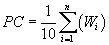
where:
W i = Dilution-weighted population from Table 4-14 for surface water body type i.
n = Number of different surface water body types in the watershed.
If PC is less than 1, do not round it to the nearest integer; if PC is 1 or more, round to the nearest integer. Enter this value for the potential contamination factor in Table 4-1.
4.1.2.3.2.5 Calculation of population factor value. Sum the factor values for Level I concentrations, Level II concentrations, and potential contamination. Do not round this sum to the nearest integer. Assign this sum as the population factor value for the watershed. Enter this value in Table 4-1.
4.1.2.3.3 Resources. To evaluate the resources factor for the watershed, select the highest value below that applies to the watershed. Assign this value as the resources factor value for the watershed. Enter this value in Table 4-1.
Assign a value of 5 if, within the in-water segment of the hazardous substance migration path for the watershed, the surface water is used for one or more of the following purposes:
- Irrigation (5 acre minimum) of commercial food crops or commercial forage crops.
- Watering of commercial livestock.
- Ingredient in commercial food preparation.
- Major or designated water recreation area, excluding drinking water use.
Assign a value of 5 if, within the in-water segment of the hazardous substance migration path for the watershed, the surface water is not used for drinking water, but either of the following applies:
- Any portion of the surface water is designated by a State for drinking water use under section 305(a) of the Clean Water Act, as amended.
- Any portion of the surface water is usable for drinking water purposes.
Assign a value of 0 if none of the above applies.
4.1.2.3.4 Calculation of drinking water threat-targets factor category value. Sum the nearest intake, population, and resources factor values for the watershed. Do not round this sum to the nearest integer. Assign this sum as the drinking water threat-targets factor category value for the watershed. Enter this value in Table 4-1.
4.1.2.4 Calculation of the drinking water threat score for a watershed. Multiply the drinking water threat factor category values for likelihood of release, waste characteristics, and targets for the watershed, and round the product to the nearest integer. Then divide by 82,500. Assign the resulting value, subject to a maximum of 100, as the drinking water threat score for the watershed. Enter this value in Table 4-1.
4.1.3 Human food chain threat. Evaluate the human food chain threat for each watershed based on three factor categories: likelihood of release, waste characteristics, and targets.
4.1.3.1 Human food chain threat-likelihood of release. Assign the same likelihood of release factor category value for the human food chain threat for the watershed as would be assigned in section 4.1.2.1.3 for the drinking water threat. Enter this value in Table 4-1.
4.1.3.2 Human food chain threat-waste characteristics. Evaluate the waste characteristics factor category for each watershed based on two factors: toxicity/persistence/bioaccumulation and hazardous waste quantity.
4.1.3.2.1 Toxicity/persistence/bioaccumulation. Evaluate all those hazardous substances eligible to be evaluated for toxicity/persistence in the drinking water threat for the watershed (see section 4.1.2.2).
4.1.3.2.1.1 Toxicity. Assign a toxicity factor value to each hazardous substance as specified in section 2.4.1.1.
4.1.3.2.1.2 Persistence. Assign a persistence factor value to each hazardous substance as specified for the drinking water threat (see section 4.1.2.2.1.2), except: use the predominant water category (that is, lakes; or rivers, oceans, coastal tidal waters, or Great Lakes) between the probable point of entry and the nearest fishery (not the nearest drinking water or resources intake) along the hazardous substance migration path for the watershed to determine which portion of Table 4-10 to use. Determine the predominant water category based on distance as specified in section 4.1.2.2.1.2. For contaminated sediments with no identified source, use the point where measurement begins rather than the probable point of entry.
4.1.3.2.1.3 Bioaccumulation potential. Use the following data hierarchy to assign a bioaccumulation potential factor value to each hazardous substance:
- Bioconcentration factor (BCF) data.
- Logarithm of the n-octanol-water partition coefficient (log K ow) data.
- Water solubility data.
Assign a bioaccumulation potential factor value to each hazardous substance from Table 4-15.
If BCF data are available for any aquatic human food chain organism for the substance being evaluated, assign the bioaccumulation potential factor value to the hazardous substance as follows:
- If BCF data are available for both fresh water and salt water for the hazardous substance, use the BCF data that correspond to the type of water body (that is, fresh water or salt water) in which the fisheries are located to assign the bioaccumulation potential factor value to the hazardous substance.
- If, however, some of the fisheries being evaluated are in fresh water and some are in salt water, or if any are in brackish water, use the BCF data that yield the higher factor value to assign the bioaccumulation potential factor value to the hazardous substance.
- If BCF data are available for either fresh water or salt water, but not for both, use the available BCF data to assign the bioaccumulation potential factor value to the hazardous substance.
If BCF data are not available for the hazardous substance, use log K ow data to assign a bioaccumulation potential factor value to organic substances, but not to inorganic substances. If BCF data are not available, and if either log K ow data are not available, the log K ow is available but exceeds 6.0, or the substance is an inorganic substance, use water solubility data to assign a bioaccumulation potential factor value.
| BCF | Assigned value |
| Greater than or equal to 10,000 | 50,000 |
| 1,000 to less than 10,000 | 5,000 |
| 100 to less than 1,000 | 500 |
| 10 to less than 100 | 50 |
| 1 to less than 10 | 5 |
| Less than 1 | 0.5 |
If BCF data are not available, and log K ow data are available and do not exceed 6.0, assign a value to an organic hazardous substance as follows (for inorganic hazardous substances, skip this step and proceed to the next):
| Log K ow | Assigned value |
| 5.5 to 6.0 | 50,000 |
| 4.5 to less than 5.5 | 5,000 |
| 3.2 to less than 4.5 | 500 |
| 2.0 to less than 3.2 | 50 |
| 0.8 to less than 2.0 | 5 |
| Less than 0.8 | 0.5 |
If BCF data are not available, and if either Log K ow data are not available, a log K ow is available but exceeds 6.0, or the substance is an inorganic substance, assign a value as follows:
| Water solubility (mg/l) | Assigned value |
| Less than 25 | 50,000 |
| 25 to 500 | 5,000 |
| Greater than 500 to 1,500 | 500 |
| Greater than 1,500 | 0.5 |
| If none of these data are available, assign a value of 0.5. | |
a Do not round to nearest integer.
b See text for use of freshwater and saltwater BCF data.
Do not distinguish between fresh water and salt water in assigning the bioaccumulation potential factor value based on log K ow or water solubility data.
If none of these data are available, assign the hazardous substance a bioaccumulation potential factor value of 0.5.
4.1.3.2.1.4 Calculation of toxicity/persistence/bioaccumulation factor value. Assign each hazardous substance a toxicity/persistence factor value from Table 4-12, based on the values assigned to the hazardous substance for the toxicity and persistence factors. Then assign each hazardous substance a toxicity/persistence/bioaccumulation factor value from Table 4-16, based on the values assigned for the toxicity/persistence and bioaccumulation potential factors. Use the hazardous substance with the highest toxicity/ persistence/bioaccumulation factor value for the watershed to assign the value to this factor. Enter this value in Table 4-1.
| Toxicity persistence factor value | Bioaccumulation potential factor value | |||||
| 50,000 | 5,000 | 500 | 50 | 5 | 0.5 | |
| 10,000 | 5×10 8 | 5×10 7 | 5×10 6 | 5×10 5 | 5×10 4 | 5,000 |
| 4,000 | 2×10 8 | 2×10 7 | 2×10 6 | 2×10 5 | 2×10 4 | 2,000 |
| 1,000 | 5×10 7 | 5×10 6 | 5×10 5 | 5×10 4 | 5,000 | 500 |
| 700 | 3.5×10 7 | 3.5×10 6 | 3.5×10 5 | 3.5×10 4 | 3,500 | 350 |
| 400 | 2×10 7 | 2×10 6 | 2×10 5 | 2×10 4 | 2,000 | 200 |
| 100 | 5×10 6 | 5×10 5 | 5×10 4 | 5,000 | 500 | 50 |
| 70 | 3.5×10 6 | 3.5×10 5 | 3.5×10 4 | 3,500 | 350 | 35 |
| 40 | 2×10 6 | 2×10 5 | 2×10 4 | 2,000 | 200 | 20 |
| 10 | 5×10 5 | 5×10 4 | 5,000 | 500 | 50 | 5 |
| 7 | 3.5×10 5 | 3.5×10 4 | 3,500 | 350 | 35 | 3.5 |
| 4 | 2×10 5 | 2×10 4 | 2,000 | 200 | 20 | 2 |
| 1 | 5×10 4 | 5,000 | 500 | 50 | 5 | 0.5 |
| 0.7 | 3.5×10 4 | 3,500 | 350 | 35 | 3.5 | 0.35 |
| 0.4 | 2×10 4 | 2,000 | 200 | 20 | 2 | 0.2 |
| 0.07 | 3,500 | 350 | 35 | 3.5 | 0.35 | 0.035 |
| 0.007 | 350 | 35 | 3.5 | 0.35 | 0.035 | 0.0035 |
| 0.0007 | 35 | 3.5 | 0.35 | 0.035 | 0.0035 | 0.00035 |
| 0 | 0 | 0 | 0 | 0 | 0 | 0 |
a Do not round to nearest integer.
4.1.3.2.2 Hazardous waste quantity. Assign the same factor value for hazardous waste quantity for the watershed as would be assigned in section 4.1.2.2.2 for the drinking water threat. Enter this value in Table 4-1.
4.1.3.2.3 Calculation of human food chain threat-waste characteristics factor category value. For the hazardous substance selected for the watershed in section 4.1.3.2.1.4, use its toxicity/persistence factor value and bioaccumulation potential factor value as follows to assign a value to the waste characteristics factor category. First, multiply the toxicity/ persistence factor value and the hazardous waste quantity factor value for the watershed, subject to a maximum product of 1x10 8. Then multiply this product by the bioaccumulation potential factor value for this hazardous substance, subject to a maximum product of 1x10 12. Based on this second product, assign a value from Table 2-7 (section 2.4.3.1) to the human food chain threat-waste characteristics factor category for the watershed. Enter this value in Table 4-1.
4.1.3.3 Human food chain threat-targets. Evaluate two target factors for each watershed: food chain individual and population. For both factors, determine whether the target fisheries are subject to actual or potential human food chain contamination.
Consider a fishery (or portion of a fishery) within the target distance limit of the watershed to be subject to actual human food chain contamination if any of the following apply:
- A hazardous substance having a bioaccumulation potential factor value of 500 or greater is present either in an observed release by direct observation to the watershed or in a surface water or sediment sample from the watershed at a level that meets the criteria for an observed release to the watershed from the site, and at least a portion of the fishery is within the boundaries of the observed release (that is, it is located either at the point of direct observation or at or between the probable point of entry and the most distant sampling point establishing the observed release).
- The fishery is closed, and a hazardous substance for which the fishery has been closed has been documented in an observed release to the watershed from the site, and at least a portion of the fishery is within the boundaries of the observed release.
- A hazardous substance is present in a tissue sample from an essentially sessile, benthic, human food chain organism from the watershed at a level that meets the criteria for an observed release to the watershed from the site, and at least a portion of the fishery is within the boundaries of the observed release.
For a fishery that meets any of these three criteria, but that is not wholly within the boundaries of the observed release, consider only the portion of the fishery that is within the boundaries of the observed release to be subject to actual human food chain contamination. Consider the remainder of the fishery within the target distance limit to be subject to potential food chain contamination.
In addition, consider all other fisheries that are partially or wholly within the target distance limit for the watershed, including fisheries partially or wholly within the boundaries of an observed release for the watershed that do not meet any of the three criteria listed above, to be subject to potential human food chain contamination. If only a portion of the fishery is within the target distance limit for the watershed, include only that portion in evaluating the targets factor category.
When a fishery (or portion of a fishery) is subject to actual food chain contamination, determine the part of the fishery subject to Level I concentrations and the part subject to Level II concentrations. If the actual food chain contamination is based on direct observation, evaluate it using Level II concentrations. However, if the actual food chain contamination is based on samples from the watershed, use these samples and, if available, additional tissue samples from aquatic human food chain organisms as specified below, to determine the part subject to Level I concentrations and the part subject to Level II concentrations:
- Determine the level of actual contamination from samples (including tissue samples from essentially sessile, benthic organisms) that meet the criteria for actual food chain contamination by comparing the exposure concentrations (see section 4.1.2.3) from these samples (or comparable samples) to the health-based benchmarks from Table 4-17, as described in section 2.5.1 and 2.5.2. Use only the exposure concentrations for those hazardous substances in the sample (or comparable samples) that meet the criteria for actual contamination of the fishery.
-
In addition, determine the level of actual contamination from other tissue samples by comparing the concentrations of hazardous substances in the tissue samples (or comparable tissue samples) to the health-based benchmarks from Table 4-17, as described in sections 2.5.1 and 2.5.2. Use only those additional tissue samples and only those hazardous substances in the tissue samples that meet all the following criteria:
- The tissue sample is from a location that is within the boundaries of the actual food chain contamination for the site (that is, either at the point of direct observation or at or between the probable point of entry and the most distant sample point meeting the criteria for actual food chain contamination).
- The tissue sample is from a species of aquatic human food chain organism that spends extended periods of time within the boundaries of the actual food chain contamination for the site and that is not an essentially sessile, benthic organism.
- The hazardous substance is a substance that is also present in a surface water, benthic, or sediment sample from within the target distance limit for the watershed and, for such a sample, meets the criteria for actual food chain contamination.
Table 4-17.—Health-Based Benchmarks for Hazardous Substances in Human Food Chain
- Concentration corresponding to Food and Drug Administration Action Level (FDAAL) for fish or shellfish.
- Screening concentration for cancer corresponding to that concentration that corresponds to the 10 -6 individual cancer risk for oral exposures.
- Screening concentration for noncancer toxicological responses corresponding to the Reference Dose (RfD) for oral exposures.
4.1.3.3.1 Food chain individual. Evaluate the food chain individual factor based on the fisheries (or portions of fisheries) within the target distance limit for the watershed. Assign this factor a value as follows:
- If any fishery (or portion of a fishery) is subject to Level I concentrations, assign a value of 50.
- If not, but if any fishery (or portion of a fishery) is subject to Level II concentrations, assign a value of 45.
- If not, but if there is an observed release of a hazardous substance having a bioaccumulation potential factor value of 500 or greater to surface water in the watershed and there is a fishery (or portion of a fishery) present anywhere within the target distance limit, assign a value of 20.
-
If there is no observed release to surface water in the watershed or there is no observed release of a hazardous substance having a bioaccumulation potential factor value of 500 or greater, but there is a fishery (or portion of a fishery) present anywhere within the target distance limit, assign a value as follows:
- Using Table 4-13, determine the highest dilution weight (that is, lowest amount of dilution) applicable to the fisheries (or portions of fisheries) within the target distance limit. Multiply this dilution weight by 20 and round to the nearest integer.
- Assign this calculated value as the factor value.
- If there are no fisheries (or portions of fisheries) within the target distance limit of the watershed, assign a value of 0.
Enter the value assigned in Table 4-1.
4.1.3.3.2 Population. Evaluate the population factor for the watershed based on three factors: Level I concentrations, Level II concentrations, and potential human food chain contamination. Determine which factor applies for a fishery (or portion of a fishery) as specified in section 4.1.3.3.
4.1.3.3.2.1 Level I concentrations. Determine those fisheries (or portions of fisheries) within the watershed that are subject to Level I concentrations.
Estimate the human food chain population value for each fishery (or portion of a fishery) as follows:
- Estimate human food chain production for the fishery based on the estimated annual production (in pounds) of human food chain organisms (for example, fish, shellfish) for that fishery, except: if the fishery is closed and a hazardous substance for which the fishery has been closed has been documented in an observed release to the fishery from a source at the site, use the estimated annual production for the period prior to closure of the fishery or use the estimated annual production from comparable fisheries that are not closed.
- Assign the fishery a value for human food chain population from Table 4- 18, based on the estimated human food production for the fishery.
- Set boundaries between fisheries at those points where human food chain production changes or where the surface water dilution weight changes.
Sum the human food chain population value for each fishery (and portion of a fishery). Multiply this sum by 10. If the product is less than 1, do not round it to the nearest integer; if 1 or more, round to the nearest integer. Assign the resulting value as the Level I concentrations factor value. Enter this value in Table 4-1.
4.1.3.3.2.2 Level II concentrations. Determine those fisheries (or portions of fisheries) within the watershed that are subject to Level II concentrations. Do not include any fisheries (or portions of fisheries) already counted under the Level I concentrations factor.
Assign each fishery (or portion of a fishery) a value for human food chain population from Table 4-18, based on the estimated human food production for the fishery. Estimate the human food chain production for the fishery as specified in section 4.1.3.3.2.1.
Sum the human food chain population value for each fishery (and portion of a fishery). If this sum is less than 1, do not round it to the nearest integer; if 1 or more, round to the nearest integer. Assign the resulting value as the Level II concentrations factor value. Enter this value in Table 4-1.
| Human food chain production (pounds per year) | Assigned human food chain population value |
| 0 | 0 |
| Greater than 0 to 100 | 0.03 |
| Greater than 100 to 1,000 | 0.3 |
| Greater than 1,000 to 10,000 | 3 |
| Greater than 10,000 to 100,000 | 31 |
| Greater than 100,000 to 1,000,000 | 310 |
| Greater than 10 6 to 10 7 | 3,100 |
| Greater than 10 7 to 10 8 | 31,000 |
| Greater than 10 8 to 10 9 | 310,000 |
| Greater than 10 9 | 3,100,000 |
a Do not round to nearest integer.
4.1.3.3.2.3 Potential human food chain contamination. Determine those fisheries (or portions of fisheries) within the watershed that are subject to potential human food chain contamination. Do not include those fisheries (or portion of fisheries) already counted under the Level I or Level II concentrations factors.
Calculate the value for the potential human food chain contamination factor (PF) for the watershed as follows:
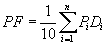
where:
P i = Human food chain population value for fishery i.
D i = Dilution weight from Table 4-13 for fishery i.
n = Number of fisheries subject to potential human food chain contamination.
In calculating PF:
- Estimate the human food chain population value (Pi) for a fishery (or portion of a fishery) as specified in section 4.1.3.3.2.1.
- Assign the fishery (or portion of a fishery) a dilution weight as indicated in Table 4-13 (section 4.1.2.3.1), except: do not assign a dilution weight of 0.5 for a "3-mile mixing zone in quiet flowing river"; instead assign a dilution weight based on the average annual flow.
If PF is less than 1, do not round it to the nearest integer; if PF is 1 or more, round to the nearest integer. Enter the value assigned in Table 4-1.
4.1.3.3.2.4 Calculation of population factor value. Sum the values for the Level I concentrations, Level II concentrations, and potential human food chain contamination factors for the watershed. Do not round this sum to the nearest integer. Assign it as the population factor value for the watershed. Enter this value in Table 4-1.
4.1.3.3.3 Calculation of human food chain threat-targets factor category value. Sum the food chain individual and population factor values for the watershed. Do not round this sum to the nearest integer. Assign it as the human food chain threat-targets factor category value for the watershed. Enter this value in Table 4-1.
4.1.3.4 Calculation of human food chain threat score for a watershed. Multiply the human food chain threat factor category values for likelihood of release, waste characteristics, and targets for the watershed, and round the product to the nearest integer. Then divide by 82,500. Assign the resulting value, subject to a maximum of 100, as the human food chain threat score for the watershed. Enter this score in Table 4-1.
4.1.4 Environmental threat. Evaluate the environmental threat for the watershed based on three factor categories: likelihood of release, waste characteristics, and targets.
4.1.4.1 Environmental threat-likelihood of release. Assign the same likelihood of release factor category value for the environmental threat for the watershed as would be assigned in section 4.1.2.1.3 for the drinking water threat. Enter this value in Table 4-1.
4.1.4.2 Environmental threat-waste characteristics. Evaluate the waste characteristics factor category for each watershed based on two factors: ecosystem toxicity/persistence/bioaccumulation and hazardous waste quantity.
4.1.4.2.1 Ecosystem toxicity/persistence/bioaccumulation. Evaluate all those hazardous substances eligible to be evaluated for toxicity/persistence in the drinking water threat for the watershed (see section 4.1.2.2).
4.1.4.2.1.1 Ecosystem toxicity. Assign an ecosystem toxicity factor value from Table 4-19 to each hazardous substance on the basis of the following data hierarchy:
- EPA chronic Ambient Water Quality Criterion (AWQC) for the substance.
- EPA chronic Ambient Aquatic Life Advisory Concentrations (AALAC) for the substance.
- EPA acute AWQC for the substance.
- EPA acute AALAC for the substance.
- Lowest LC 50 value for the substance.
In assigning the ecosystem toxicity factor value to the hazardous substance:
- If either an EPA chronic AWQC or AALAC is available for the hazardous substance, use it to assign the ecosystem toxicity factor value. Use the chronic AWQC in preference to the chronic AALAC when both are available.
- If neither is available, use the EPA acute AWQC or AALAC to assign the ecosystem toxicity factor value. Use the acute AWQC in preference to the acute AALAC.
- If none of the chronic and acute AWQCs and AALACs is available, use the lowest LC 50 value to assign the ecosystem toxicity factor value.
- If an LC50 value is also not available, assign an ecosystem toxicity factor value of 0 to the hazardous substance and use other hazardous substances for which data are available in evaluating the pathway.
If an ecosystem toxicity factor value of 0 is assigned to all hazardous substances eligible to be evaluated for the watershed (that is, insufficient data are available for evaluating all the substances), use a default value of 100 as the ecosystem toxicity factor value for all these hazardous substances.
With regard to the AWQC, AALAC, or LC 50 selected for assigning the ecosystem toxicity factor value to the hazardous substance:
- If values for the selected AWQC, AALAC, or LC 50 are available for both fresh water and marine water for the hazardous substance, use the value that corresponds to the type of water body (that is, fresh water or salt water) in which the sensitive environments are located to assign the ecosystem toxicity factor value to the hazardous substance.
- If, however, some of the sensitive environments being evaluated are in fresh water and some are in salt water, or if any are in brackish water, use the value (fresh water or marine) that yields the higher factor value to assign the ecosystem toxicity factor value to the hazardous substance.
- If a value for the selected AWQC, AALAC, or LC 50 is available for either fresh water or marine water, but not for both, use the available one to assign an ecosystem toxicity factor value to the hazardous substance.
| EPA chronic AWQC or AALAC | Assigned value |
| Less than 1 µg/l | 10,000 |
| 1 to 10 µg/l | 1,000 |
| Greater than 10 to 100 µg/l | 100 |
| Greater than 100 to 1,000 µg/l | 10 |
| Greater than 1,000 µg/l | 1 |
| If neither an EPA chronic AWQC nor EPA chronic AALAC is available, assign a value based on the EPA acute AWQC or AALAC as follows: c | |
| EPA acute AWQC or AALAC | Assigned value |
| Less than 100 µg/l | 10,000 |
| 100 to 1,000 µg/l | 1,000 |
| Greater than 1,000 to 10,000 µg/l | 100 |
| Greater than 10,000 to 100,000 µg/l | 10 |
| Greater than 100,000 µg/l | 1 |
| If neither an EPA chronic or acute AWQC nor EPA chronic or acute AALAC is available, assign a value from the LC 50 as follows: | |
| LC 50 | Assigned value |
| Less than 100 µg/l | 10,000 |
| 100 to 1,000 µg/l | 1,000 |
| Greater than 1,000 to 10,000 µg/l | 100 |
| Greater than 10,000 to 100,000 µg/l | 10 |
| Greater than 100,000 µg/l | 1 |
| If none of the AWQCs and AALACs nor the LC 50 is available, assign a value of 0. | |
a AWQC—Ambient Water Quality Criteria.
b AALAC—Ambient Aquatic Life Advisory Concentrations.
c Use the AWQC value in preference to the AALAC when both are available. See text for use of fresh water and marine values.
4.1.4.2.1.2 Persistence. Assign a persistence factor value to each hazardous substance as specified in section 4.1.2.2.1.2, except: use the predominant water category (that is lakes; or rivers, oceans, coastal tidal waters, or Great Lakes) between the probable point of entry and the nearest sensitive environment (not the nearest drinking water or resources intake) along the hazardous substance migration path for the watershed to determine which portion of Table 4-10 to use. Determine the predominant water category based on distance as specified in section 4.1.2.2.1.2. For contaminated sediments with no identified source, use the point where measurement begins rather than the probable point of entry.
4.1.4.2.1.3 Ecosystem bioaccumulation potential. Assign an ecosystem bioaccumulation potential factor value to each hazardous substance in the same manner specified for the bioaccumulation potential factor in section 4.1.3.2.1.3, except:
- Use BCF data for all aquatic organisms, not just for aquatic human food chain organisms.
- Use the BCF data that corresponds to the type of water body (that is, fresh water or salt water) in which the sensitive environments (not fisheries) are located.
4.1.4.2.1.4 Calculation of ecosystem toxicity/persistence/bioaccumulation factor value. Assign each hazardous substance an ecosystem toxicity/ persistence factor value from Table 4-20, based on the values assigned to the hazardous substance for the ecosystem toxicity and persistence factors. Then assign each hazardous substance an ecosystem toxicity/persistence/ bioaccumulation factor value from Table 4-21, based on the values assigned for the ecosystem toxicity/persistence and ecosystem bioaccumulation potential factors. Select the hazardous substance with the highest ecosystem toxicity/persistence/bioaccumulation factor value for the watershed and use it to assign the value to this factor. Enter this value in Table 4-1.
| Persistence factor value | Ecosystem toxicity factor value | |||||
| 10,000 | 1,000 | 100 | 10 | 1 | 0 | |
| 1.0 | 10,000 | 1,000 | 100 | 10 | 1 | 0 |
| 0.4 | 4,000 | 400 | 40 | 4 | 0.4 | 0 |
| 0.07 | 700 | 70 | 7 | 0.7 | 0.07 | 0 |
| 0.0007 | 7 | 0.7 | 0.07 | 0.007 | 0.0007 | 0 |
a Do not round to nearest integer.
| Ecosystem toxicity persistence factor value | Ecosystem bioaccumulation potential factor value | |||||
| 50,000 | 5,000 | 500 | 50 | 5 | 0.5 | |
| 10,000 | 5×10 8 | 5×10 7 | 5×10 6 | 5×10 5 | 5×10 4 | 5,000 |
| 4,000 | 2×10 8 | 2×10 7 | 2×10 6 | 2×10 5 | 2×10 4 | 2,000 |
| 1,000 | 5×10 7 | 5×10 6 | 5×10 5 | 5×10 4 | 5,000 | 500 |
| 700 | 3.5×10 7 | 3.5×10 6 | 3.5×10 5 | 3.5×10 4 | 3,500 | 350 |
| 400 | 2×10 7 | 2×10 6 | 2×10 5 | 2×10 4 | 2,000 | 200 |
| 100 | 5×10 6 | 5×10 5 | 5×10 4 | 5,000 | 500 | 50 |
| 70 | 3.5×10 6 | 3.5×10 5 | 3.5×10 4 | 3,500 | 350 | 35 |
| 40 | 2×10 6 | 2×10 5 | 2×10 4 | 2,000 | 200 | 20 |
| 10 | 5×10 5 | 5×10 4 | 5,000 | 500 | 50 | 5 |
| 7 | 3.5×10 5 | 3.5×10 4 | 3,500 | 350 | 35 | 3.5 |
| 4 | 2×10 5 | 2×10 4 | 2,000 | 200 | 20 | 2 |
| 1 | 5×10 4 | 5,000 | 500 | 50 | 5 | 0.5 |
| 0.7 | 3.5×10 4 | 3,500 | 350 | 35 | 3.5 | 0.35 |
| 0.4 | 2×10 4 | 2,000 | 200 | 20 | 2 | 0.2 |
| 0.07 | 3,500 | 350 | 35 | 3.5 | 0.35 | 0.035 |
| 0.007 | 350 | 35 | 3.5 | 0.35 | 0.035 | 0.0035 |
| 0.0007 | 35 | 3.5 | 0.35 | 0.035 | 0.0035 | 0.00035 |
| 0 | 0 | 0 | 0 | 0 | 0 | 0 |
a Do not round to nearest integer.
4.1.4.2.2 Hazardous waste quantity. Assign the same factor value for hazardous waste quantity for the watershed as would be assigned in section 4.1.2.2.2 for the drinking water threat. Enter this value in Table 4-1.
4.1.4.2.3 Calculation of environmental threat-waste characteristics factor category value. For the hazardous substance selected for the watershed in section 4.1.4.2.1.4, use its ecosystem toxicity/persistence factor value and ecosystem bioaccumulation potential factor value as follows to assign a value to the waste characteristics factor category. First, multiply the ecosystem toxicity/persistence factor value and the hazardous waste quantity factor value for the watershed, subject to a maximum product of 1x10 8. Then multiply this product by the ecosystem bioaccumulation potential factor value for this hazardous substance, subject to a maximum product of 1x10 12. Based on this second product, assign a value from Table 2-7 (section 2.4.3.1) to the environmental threat-waste characteristics factor category for the watershed. Enter this value in Table 4-1.
Table 4-22.—Ecological-Based Benchmarks for Hazardous Substances in Surface Water
- Concentration corresponding to EPA Ambient Water Quality Criteria (AWQC) for protection of aquatic life (fresh water or marine).
- Concentration corresponding to EPA Ambient Aquatic Life Advisory Concentrations (AALAC).
-
Select the appropriate AWQC and AALAC as follows:
- Use chronic value, if available; otherwise use acute value.
- If the sensitive environment being evaluated is in fresh water, use fresh water value, except: if no fresh water value is available, use marine value if available.
- If the sensitive environment being evaluated is in salt water, use marine value, except: if no marine value is available, use fresh water value if available.
- If the sensitive environment being evaluated is in both fresh water and salt water, or is in brackish water, use lower of fresh water or marine values.
| Sensitive environment | Assigned value |
| Critical habitat a for Federal designated endangered or threatened species | 100 |
| Marine Sanctuary | |
| National Park | |
| Designated Federal Wilderness Area | |
| Areas identified under Coastal Zone Management Act b | |
| Sensitive areas identified under National Estuary Program c or Near Coastal Waters Program d | |
| Critical areas identified under the Clean Lakes Program e | |
| National Monument f | |
| National Seashore Recreational Area | |
| National Lakeshore Recreational Area | |
| Habitat known to be used by Federal designated or proposed endangered or threatened species | 75 |
| National Preserve | |
| National or State Wildlife Refuge | |
| Unit of Coastal Barrier Resources System | |
| Coastal Barrier (undeveloped) | |
| Federal land designated for protection of natural ecosystems | |
| Administratively Proposed Federal Wilderness Area | |
| Spawning areas critical g for the maintenance of fish/shellfish species within river, lake, or coastal tidal waters | |
| Migratory pathways and feeding areas critical for maintenance of anadromous fish species within river reaches or areas in lakes or coastal tidal waters in which the fish spend extended periods of time | |
| Terrestrial areas utilized for breeding by large or dense aggregations of animals h | |
| National river reach designated as Recreational | |
| Habitat known to be used by State designated endangered or threatened species | 50 |
| Habitat known to be used by species under review as to its Federal endangered or threatened status | |
| Coastal Barrier (partially developed) | |
| Federal designated Scenic or Wild River | |
| State land designated for wildlife or game management | 25 |
| State designated Scenic or Wild River | |
| State designated Natural Areas | |
| Particular areas, relatively small in size, important to maintenance of unique biotic communities | |
| State designated areas for protection or maintenance of aquatic life i | 5 |
a Critical habitat as defined in 50 CFR 424.02.
b Areas identified in State Coastal Zone Management plans as requiring protection because of ecological value.
c National Estuary Program study areas (subareas within estuaries) identified in Comprehensive Conservation and Management Plans as requiring protection because they support critical life stages of key estuarine species (Section 320 of Clean Water Act, as amended).
d Near Coastal Waters as defined in Sections 104(b)(3), 304(1), 319, and 320 of Clean Water Act, as amended.
e Clean Lakes Program critical areas (subareas within lakes, or in some cases entire small lakes) identified by State Clean Lake Plans as critical habitat (Section 314 of Clean Water Act, as amended).
f Use only for air migration pathway.
g Limit to areas described as being used for intense or concentrated spawning by a given species.
h For the air migration pathway, limit to terrestrial vertebrate species. For the surface water migration pathway, limit to terrestrial vertebrate species with aquatic or semiaquatic foraging habits.
i Areas designated under Section 305(a) of Clean Water Act, as amended.
| Total length of wetlands a (miles) | Assigned value |
| Less than 0.1 | 0 |
| 0.1 to 1 | 25 |
| Greater than 1 to 2 | 50 |
| Greater than 2 to 3 | 75 |
| Greater than 3 to 4 | 100 |
| Greater than 4 to 8 | 150 |
| Greater than 8 to 12 | 250 |
| Greater than 12 to 16 | 350 |
| Greater than 16 to 20 | 450 |
| Greater than 20 | 500 |
a Wetlands as defined in 40 CFR section 230.3.
4.1.4.3 Environmental threat-targets. Evaluate the environmental threat- targets factor category for a watershed using one factor: sensitive environments.
4.1.4.3.1 Sensitive environments. Evaluate sensitive environments along the hazardous substance migration path for the watershed based on three factors: Level I concentrations, Level II concentrations, and potential contamination.
Determine which factor applies to each sensitive environment as specified in section 4.1.2.3, except: use ecological-based benchmarks (Table 4-22) rather than health-based benchmarks (Table 3-10) in determining the level of contamination from samples. In determining the level of actual contamination, use a point of direct observation anywhere within the sensitive environment or samples (that is, surface water, benthic, or sediment samples) taken anywhere within or beyond the sensitive environment (or anywhere adjacent to or beyond the sensitive environment if it is contiguous to the migration path).
4.1.4.3.1.1 Level I concentrations. Assign value(s) from Table 4-23 to each sensitive environment subject to Level I concentrations.
For those sensitive environments that are wetlands, assign an additional value from Table 4-24. In assigning a value from Table 4-24, include only those portions of wetlands located along the hazardous substance migration path in the area of Level I concentrations. If a wetland is located partially along the area of Level I concentrations and partially along the area of Level II concentrations and/or potential contamination, then solely for purposes of Table 4-24, count the portion(s) along the areas of Level II concentrations or potential contamination under the Level II concentrations factor (section 4.1.4.3.1.2) or potential contamination factor (section 4.1.4.3.1.3), as appropriate.
Estimate the total length of wetlands along the hazardous substance migration path (that is, wetland frontage) in the area of Level I concentrations and assign a value from Table 4-24 based on this total length. Estimate this length as follows:
- For an isolated wetland or for a wetland where the probable point of entry to surface water is in the wetland, use the perimeter of that portion of the wetland subject to Level I concentrations as the length.
- For rivers, use the length of the wetlands contiguous to the in-water segment of the hazardous substance migration path (that is, wetland frontage).
- For lakes, oceans, coastal tidal waters, and Great Lakes, use the length of the wetlands along the shoreline within the target distance limit (that is, wetland frontage along the shoreline).
Calculate the Level I concentrations factor value (SH) for the watershed as follows:
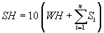
where:
WH = Value assigned from Table 4-24 to wetlands along the area of Level I concentrations.
S i = Value(s) assigned from Table 4-23 to sensitive environment i.
n = Number of sensitive environments from Table 4-23 subject to Level I concentrations.
Enter the value assigned in Table 4-1.
4.1.4.3.1.2 Level II concentrations. Assign value(s) from Table 4-23 to each sensitive environment subject to Level II concentrations. Do not include sensitive environments already counted for Table 4-23 under the Level I concentrations factor for this watershed.
For those sensitive environments that are wetlands, assign an additional value from Table 4-24. In assigning a value from Table 4-24, include only those portions of wetlands located along the hazardous substance migration path in the area of Level II concentrations, as specified in section 4.1.4.3.1.1.
Estimate the total length of wetlands along the hazardous substance migration path (that is, wetland frontage) in the area of Level II concentrations and assign a value from Table 4-24 based on this total length. Estimate this length as specified in section 4.1.4.3.1.1, except: for an isolated wetland or for a wetland where the probable point of entry to surface water is in the wetland, use the perimeter of that portion of the wetland subject to Level II (not Level I) concentrations as the length.
Calculate the Level II concentrations value (SL) for the watershed as follows:
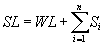
where:
WL = Value assigned from Table 4-24 to wetlands along the area of Level II concentrations.
Si = Value(s) assigned from Table 4-23 to sensitive environment i.
n = Number of sensitive environments from Table 4-23 subject to Level II concentrations.
Enter the value assigned in Table 4-1.
4.1.4.3.1.3 Potential contamination. Assign value(s) from Table 4-23 to each sensitive environment subject to potential contamination. Do not include sensitive environments already counted for Table 4-23 under the Level I or Level II concentrations factors.
For each type of surface water body in Table 4-13 (section 4.1.2.3.1), sum the value(s) assigned from Table 4-23 to the sensitive environments along that type of surface water body, except: do not use the surface water body type "3-mile mixing zone in quiet flowing river." If a sensitive environment is along two or more types of surface water bodies (for example, Wildlife Refuge contiguous to both a moderate stream and a large river), assign the sensitive environment only to that surface water body type having the highest dilution weight value from Table 4-13.
For those sensitive environments that are wetlands, assign an additional value from Table 4-24. In assigning a value from Table 4-24, include only those portions of wetlands located along the hazardous substance migration path in the area of potential contamination, as specified in section 4.1.4.3.1.1. Aggregate these wetlands by type of surface water body, except: do not use the surface water body type "3-mile mixing zone in quiet flowing river." Treat the wetlands aggregated within each type of surface water body as separate sensitive environments solely for purposes of applying Table 4- 24. Estimate the total length of the wetlands within each surface water body type as specified in section 4.1.4.3.1.1, except: for an isolated wetland or for a wetland where the probable point of entry to surface water is in the wetland, use the perimeter of that portion of the wetland subject to potential contamination (or the portion of that perimeter that is within the target distance limit) as the length. Assign a separate value from Table 4-24 for each type of surface water body in the watershed.
Calculate the potential contamination factor value (SP) for the watershed as follows:
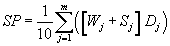
where:

S ij = Value(s) assigned from table 4–23 to sensitive environment i in surface water body type j.
n = Number of sensitive environments from table 4–23 subject to potential contamination.
W j = Value assigned from table 4–24 for wetlands along the area of potential contamination in surface water body type j.
D j = Dilution weight from table 4–13 for surface water body type j.
m = Number of different surface water body types from table 4–13 in the watershed.
If SP is less than 1, do not round it to the nearest integer; if SP is 1 or more, round to the nearest integer. Enter this value for the potential contamination factor in Table 4-1.
4.1.4.3.1.4 Calculation of environmental threat-targets factor category value. Sum the values for the Level I concentrations, Level II concentrations, and potential contamination factors for the watershed. Do not round this sum to the nearest integer. Assign this sum as the environmental threat-targets factor category value for the watershed. Enter this value in Table 4-1.
4.1.4.4 Calculation of environmental threat score for a watershed. Multiply the environmental threat factor category values for likelihood of release, waste characteristics, and targets for the watershed, and round the product to the nearest integer. Then divide by 82,500. Assign the resulting value, subject to a maximum of 60, as the environmental threat score for the watershed. Enter this score in Table 4-1.
4.1.5 Calculation of overland/flood migration component score for a watershed. Sum the scores for the three threats for the watershed (that is, drinking water, human food chain, and environmental threats). Assign the resulting score, subject to a maximum value of 100, as the surface water overland/flood migration component score for the watershed. Enter this score in Table 4-1.
4.1.6 Calculation of overland/flood migration component score. Select the highest surface water overland/flood migration component score from the watersheds evaluated. Assign this score as the surface water overland/flood migration component score for the site, subject to a maximum score of 100. Enter this score in Table 4-1.
4.2 Ground water to surface water migration component. Use the ground water to surface water migration component to evaluate surface water threats that result from migration of hazardous substances from a source at the site to surface water via ground water. Evaluate three types of threats for this component: drinking water threat, human food chain threat, and environmental threat.
4.2.1 General considerations.
4.2.1.1 Eligible surface waters. Calculate ground water to surface water migration component scores only for surface waters (see section 4.0.2) for which all the following conditions are met:
- A portion of the surface water is within 1 mile of one or more sources at the site having a containment factor value greater than 0 (see section 4.2.2.1.2).
- No aquifer discontinuity is established between the source and the portion of the surface water within 1 mile of the source (see section 3.0.1.2.2). However, if hazardous substances have migrated across an apparent discontinuity within this 1 mile distance, do not consider a discontinuity present in scoring the site.
- The top of the uppermost aquifer is at or above the bottom of the surface water.
Do not evaluate this component for sites consisting solely of contaminated sediments with no identified source.
4.2.1.2 Definition of hazardous substance migration path for ground water to surface water migration component. The hazardous substance migration path includes both the ground water segment and the surface water in-water segment that hazardous substances would take as they migrate away from sources at the site:
- Restrict the ground water segment to migration via the uppermost aquifer between a source and the surface water.
-
Begin the surface water in-water segment at the probable point of entry from the uppermost aquifer to the surface water. Identify the probable point of entry as that point of the surface water that yields the shortest straight-line distance, within the aquifer boundary (see section 3.0.1.2), from the sources at the site with a containment factor value greater than 0 to the surface water.
- For rivers, continue the in-water segment in the direction of flow (including any tidal flows) for the distance established by the target distance limit (see section 4.2.1.4).
- For lakes, oceans, coastal tidal waters, or Great Lakes, do not consider flow direction. Instead apply the target distance limit as an arc.
- If the in-water segment includes both rivers and lakes (or oceans, coastal tidal waters, or Great Lakes), apply the target distance limit to their combined in-water segments.
Consider a site to be in two or more watersheds for this component if two or more hazardous substance migration paths from the sources at the site do not reach a common point within the target distance limit. If the site is in more than one watershed, define a separate hazardous substance migration path for each watershed. Evaluate the ground water to surface water migration component for each watershed separately as specified in section 4.2.1.5.
4.2.1.3 Observed release of a specific hazardous substance to surface water in-water segment. Section 4.2.2.1.1 specifies the criteria for assigning values to the observed release factor for the ground water to surface water migration component. With regard to an individual hazardous substance, consider an observed release of that hazardous substance to be established for the surface water in-water segment of the ground water to surface water migration component only when the hazardous substance meets the criteria both for an observed release both to ground water (see section 4.2.2.1.1) and for an observed release by chemical analysis to surface water (see section 4.1.2.1.1).
If the hazardous substance meets the section 4.1.2.1.1 criteria for an observed release by chemical analysis to surface water but does not also meet the criteria for an observed release to ground water, do not use any samples of that hazardous substance from the surface water in-water segment in evaluating the factors of this component (for example, do not use the hazardous substance in establishing targets subject to actual contamination or in determining the level of actual contamination for a target).
4.2.1.4 Target distance limit. Determine the target distance limit for each watershed as specified in section 4.1.1.2, except: do not extend the target distance limit to a sample location beyond 15 miles unless at least one hazardous substance in a sample from that location meets the criteria in section 4.2.1.3 for an observed release to the surface water in-water segment.
Determine the targets eligible to be evaluated for each watershed and establish whether these targets are subject to actual or potential contamination as specified in section 4.1.1.2, except: do not establish actual contamination based on a sample location unless at least one hazardous substance in a sample from that location meets the criteria in section 4.2.1.3 for an observed release to the surface water in-water segment.
4.2.1.5 Evaluation of ground water to surface water migration component. Evaluate the drinking water threat, human food chain threat, and environmental threat for each watershed for this component based on three factor categories: likelihood of release, waste characteristics, and targets. Figure 4-2 indicates the factors included within each factor category for each type of threat.
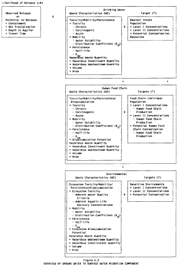
Determine the ground water to surface water migration component score (Sgs) for a watershed in terms of the factor category values as follows:
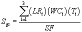
where:
LR i = Likelihood of release factor category value for threat i (that is, drinking water, human food chain, or environmental threat).
WC i = Waste characteristics factor category value for threat i.
T i = Targets factor category value for threat i.
sf = Scaling factor.
Table 4-25 outlines the specific calculation procedure.
If the site is in only one watershed, assign the ground water to surface water migration component score for that watershed as the ground water to surface water migration component score for the site.
If the site is in more than one watershed:
- Calculate a separate ground water to surface water migration component score for each watershed, using likelihood of release, waste characteristics, and targets applicable to each watershed.
- Select the highest ground water to surface water migration component score from the watersheds evaluated and assign it as the ground water to surface water migration component score for the site.
| Factor categories and factors | Maximum value | Value assigned |
| Drinking Water Threat | ||
| Likelihood of Release to Aquifer: | ||
| 1. Observed Release | 550 | ___ |
| 2. Potential to Release: | ||
| 2a. Containment | 10 | ___ |
| 2b. Net Precipitation | 10 | ___ |
| 2c. Depth to Aquifer | 5 | ___ |
| 2d. Travel Time | 35 | ___ |
| 2e. Potential to Release (lines 2a[2b+2c+2d]) | 500 | ___ |
| 3. Likelihood of Release (higher of lines 1 and 2e) | 550 | ___ |
| Waste Characteristics: | ||
| 4. Toxicity/Mobility/Persistence | (a) | ___ |
| 5. Hazardous Waste Quantity | (a) | ___ |
| 6. Waste Characteristics | 100 | ___ |
| Targets: | ||
| 7. Nearest Intake | 50 | ___ |
| 8. Population | ||
| 8a. Level I Concentrations | (b) | ___ |
| 8b. Level II Concentrations | (b) | ___ |
| 8c. Potential Contamination | (b) | ___ |
| 8d. Population (lines 8a + 8b + 8c) | ___ | |
| 9. Resources | 5 | ___ |
| 10. Targets (lines 7 + 8d + 9) | (b) | ___ |
| Drinking Water Threat Score: | ||
| 11. Drinking Water Threat Score ([lines 3×6×10]/82,500, subject to a maximum of 100) | 100 | ___ |
| Human Food Chain Threat | ||
| Likelihood of Release: | ||
| 12. Likelihood of Release (same value as line 3) | 550 | ___ |
| Waste Characteristics: | ||
| 13. Toxicity/Mobility/Persistence/Bioaccumulation | (a) | ___ |
| 14. Hazardous Waste Quantity | (a) | ___ |
| 15. Waste Characteristics | 1,000 | ___ |
| Targets: | ||
| 16. Food Chain Individual | 50 | ___ |
| 17. Population: | ||
| 17a. Level I Concentrations | (b) | ___ |
| 17b. Level II Concentrations | (b) | ___ |
| 17c. Potential Human Food Chain Contamination | (b) | ___ |
| 17d. Population (lines 17a + 17b + 17c) | (b) | ___ |
| 18. Targets (Lines 16 + 17d) | (b) | ___ |
| Human Food Chain Threat Score: | ||
| 19. Human Food Chain Threat Score ([lines 12×15×18]/82,500, subject to a maximum of 100) | 100 | ___ |
| Environmental Threat | ||
| Likelihood of Release: | ||
| 20. Likelihood of Release (same value as line 3) | 550 | ___ |
| Waste Characteristics: | ||
| 21. Ecosystem Toxicity/Mobility/Persistence/Bioaccumulation | (a) | ___ |
| 22. Hazardous Waste Quantity | (a) | ___ |
| 23. Waste Characteristics | 1,000 | ___ |
| Targets: | ||
| 24. Sensitive Environments: | ||
| 24a. Level I Concentrations | (b) | ___ |
| 24b. Level II Concentrations | (b) | ___ |
| 24c. Potential Contamination | (b) | ___ |
| 24d. Sensitive Environments (lines 24a + 24b + 24c) | (b) | ___ |
| 25. Targets (value from line 24d) | (b) | ___ |
| Environmental Threat Score: | ||
| 26. Environmental Threat Score ([lines 20×23×25]/82,500, subject to a maximum of 60) | 60 | ___ |
| Ground Water to Surface Water Migration Component Score for a Watershed | ||
| 27. Watershed Score c (lines 11 + 19 + 26, subject to a maximum of 100) | 100 | ___ |
| 28. Component Score (S gs) c (highest score from Line 27 for all watersheds evaluated, subject to a maximum of 100) | 100 | ___ |
a Maximum value applies to waste characteristics category.
b Maximum value not applicable.
c Do not round to nearest integer.
4.2.2 Drinking water threat. Evaluate the drinking water threat for each watershed based on three factor categories: likelihood of release, waste characteristics, and targets.
4.2.2.1 Drinking water threat-likelihood of release. Evaluate the likelihood of release factor category for each watershed in terms of an observed release factor or a potential to release factor.
4.2.2.1.1 Observed release. Establish an observed release to the uppermost aquifer as specified in section 3.1.1. If an observed release can be established for the uppermost aquifer, assign an observed release factor value of 550 to that watershed, enter this value in Table 4-25, and proceed to section 4.2.2.1.3. If no observed release can be established, assign an observed release factor value of 0, enter this value in Table 4-25, and proceed to section 4.2.2.1.2.
4.2.2.1.2 Potential to release. Evaluate potential to release only if an observed release cannot be established for the uppermost aquifer. Calculate a potential to release value for the uppermost aquifer as specified in section 3.1.2 and sections 3.1.2.1 through 3.1.2.5. Assign the potential to release value for the uppermost aquifer as the potential to release factor value for the watershed. Enter this value in Table 4-25.
4.2.2.1.3 Calculation of drinking water threat-likelihood of release factor category value. If an observed release is established for the uppermost aquifer, assign the observed release factor value of 550 as the likelihood of release factor category value for the watershed. Otherwise, assign the potential to release factor value as the likelihood of release factor category value for the watershed. Enter the value assigned in Table 4- 25.
4.2.2.2 Drinking water threat-waste characteristics. Evaluate the waste characteristics factor category for each watershed based on two factors: toxicity/mobility/persistence and hazardous waste quantity. Evaluate only those hazardous substances available to migrate from the sources at the site to the uppermost aquifer (see section 3.2). Such hazardous substances include:
- Hazardous substances that meet the criteria for an observed release to ground water.
- All hazardous substances associated with a source that has a ground water containment factor value greater than 0 (see sections 2.2.2, 2.2.3, and 3.1.2.1).
4.2.2.2.1 Toxicity/mobility/persistence. For each hazardous substance, assign a toxicity factor value, a mobility factor value, a persistence factor value, and a combined toxicity/mobility/persistence factor value as specified in sections 4.2.2.2.1.1 through 4.2.2.2.1.4.
4.2.2.2.1.1 Toxicity. Assign a toxicity factor value to each hazardous substance as specified in section 2.4.1.1.
4.2.2.2.1.2 Mobility. Assign a ground water mobility factor value to each hazardous substance as specified in section 3.2.1.2.
4.2.2.2.1.3 Persistence. Assign a surface water persistence factor value to each hazardous substance as specified in section 4.1.2.2.1.2.
4.2.2.2.1.4 Calculation of toxicity/mobility/persistence factor value. First, assign each hazardous substance a toxicity/mobility factor value from Table 3-9 (section 3.2.1.3), based on the values assigned to the hazardous substance for the toxicity and mobility factors. Then assign each hazardous substance a toxicity/mobility/persistence factor value from Table 4-26, based on the values assigned for the toxicity/mobility and persistence factors. Use the substance with the highest toxicity/mobility/ persistence factor value for the watershed to assign the value to this factor. Enter this value in Table 4-25.
4.2.2.2.2 Hazardous waste quantity. Assign the same factor value for hazardous waste quantity for the watershed as would be assigned for the uppermost aquifer in section 3.2.2. Enter this value in Table 4-25.
4.2.2.2.3 Calculation of drinking water threat-waste characteristics factor category value. Multiply the toxicity/mobility/persistence and hazardous waste quantity factor values for the watershed, subject to a maximum product of 1x10 8. Based on this product, assign a value from Table 2- 7 (section 2.4.3.1) to the drinking water threat-waste characteristics factor category for the watershed. Enter this value in Table 4-25.
4.2.2.3 Drinking water threat-targets. Evaluate the targets factor category for each watershed based on three factors: nearest intake, population, and resources.
| Toxicity/mobility factor value | Persistence factor value | |||
| 1.0 | 0.4 | 0.07 | 0.0007 | |
| 10,000 | 10,000 | 4,000 | 700 | 7 |
| 2,000 | 2,000 | 800 | 140 | 1.4 |
| 1,000 | 1,000 | 400 | 70 | 0.7 |
| 200 | 200 | 80 | 14 | 0.14 |
| 100 | 100 | 40 | 7 | 0.07 |
| 20 | 20 | 8 | 1.4 | 0.014 |
| 10 | 10 | 4 | 0.7 | 0.007 |
| 2 | 2 | 0.8 | 0.14 | 0.0014 |
| 1 | 1 | 0.4 | 0.07 | 7×10 −4 |
| 0.2 | 0.2 | 0.08 | 0.014 | 1.4×10 −4 |
| 0.1 | 0.1 | 0.04 | 0.007 | 7×10 −5 |
| 0.02 | 0.02 | 0.008 | 0.0014 | 1.4×10 −5 |
| 0.01 | 0.01 | 0.004 | 7×10 −4 | 7×10 −6 |
| 0.002 | 0.002 | 8×10 −4 | 1.4×10 −4 | 1.4×10 −6 |
| 0.001 | 0.001 | 4×10 −4 | 7×10 −5 | 7×10 −7 |
| 2×10 −4 | 2×10 −4 | 8×10 −5 | 1.4×10 −5 | 1.4×10 −7 |
| 1×10 −4 | 1×10 −4 | 4×10 −5 | 7×10 −6 | 7×10 −8 |
| 2×10 −5 | 2×10 −5 | 8×10 −6 | 1.4×10 −6 | 1.4×10 −8 |
| 2×10 −6 | 2×10 −6 | 8×10 −7 | 1.4×10 −7 | 1.4×10 −9 |
| 2×10 −7 | 2×10 −7 | 8×10 −8 | 1.4×10 −8 | 1.4×10 −10 |
| 2×10 −8 | 2×10 −8 | 8×10 −9 | 1.4×10 −9 | 1.4×10 −11 |
| 2×10 −9 | 2×10 −9 | 8×10 −10 | 1.4×10 −10 | 1.4×10 −12 |
| 0 | 0 | 0 | 0 | 0 |
a Do not round to nearest integer.
For the nearest intake and population factors, determine whether the target surface water intakes are subject to actual or potential contamination as specified in section 4.1.1.2, subject to the restrictions specified in sections 4.2.1.3 and 4.2.1.4.
When the intake is subject to actual contamination, evaluate it using Level I concentrations or Level II concentrations. Determine which level applies for the intake by comparing the exposure concentrations from a sample (or comparable samples) to health-based benchmarks as specified in section 4.1.2.3, except use only those samples from the surface water in-water segment and only those hazardous substances in such samples that meet the conditions in sections 4.2.1.3 and 4.2.1.4.
4.2.2.3.1 Nearest intake. Assign a value to the nearest intake factor as specified in section 4.1.2.3.1 with the following modification. For the intake being evaluated, multiply its dilution weight from Table 4-13 (section 4.1.2.3.1) by a value selected from Table 4-27. Use the resulting product, not the value from Table 4-13, as the dilution weight for the intake for the ground water to surface water component. Do not round this product to the nearest integer.
Select the value from Table 4-27 based on the angle Θ, the angle defined by the sources at the site and either the two points at the intersection of the surface water body and the 1-mile distance ring of any two other points of the surface water body within the 1-mile distance ring, whichever results in the largest angle. (See Figure 4-3 for an example of how to determine Θ.) If the surface water body does not extend to the 1-mile ring at one or both ends, define Θ using the surface water endpoint(s) within the 1-mile ring or any two other points of the surface water body within the 1-mile distance ring, whichever results in the largest angle.
| Angle Θ (degrees) | Assigned value a |
| 0 | 0 |
| Greater than 0 to 18 | 0.05 |
| Greater than 18 to 54 | 0.1 |
| Greater than 54 to 90 | 0.2 |
| Greater than 90 to 126 | 0.3 |
| Greater than 126 to 162 | 0.4 |
| Greater than 162 to 198 | 0.5 |
| Greater than 198 to 234 | 0.6 |
| Greater than 234 to 270 | 0.7 |
| Greater than 270 to 306 | 0.8 |
| Greater than 306 to 342 | 0.9 |
| Greater than 342 to 360 | 1.0 |
a Do not round to nearest integer.
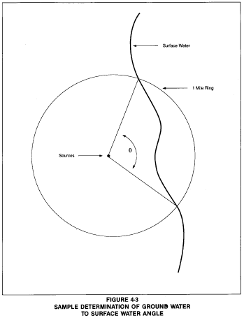
| Toxicity/mobility/persistence factor value | Bioaccumlation potential factor value | |||||
| 50,000 | 5,000 | 500 | 50 | 5 | 0.5 | |
| 10,000 | 5×10 8 | 5×10 7 | 5×10 6 | 5×10 5 | 5×10 4 | 5,000 |
| 4,000 | 2×10 8 | 2×10 7 | 2×10 6 | 2×10 5 | 2×10 4 | 2,000 |
| 2,000 | 1×10 8 | 1×10 7 | 1×10 6 | 1×10 5 | 1×10 4 | 1,000 |
| 1,000 | 5×10 7 | 5×10 6 | 5×10 5 | 5×10 4 | 5,000 | 500 |
| 800 | 4×10 7 | 4×10 6 | 4×10 5 | 4×10 4 | 4,000 | 400 |
| 700 | 3.5×10 7 | 3.5×10 6 | 3.5×10 5 | 3.5×10 4 | 3,500 | 350 |
| 400 | 2×10 7 | 2×10 6 | 2×10 5 | 2×10 4 | 2,000 | 200 |
| 200 | 1×10 7 | 1×10 6 | 1×10 5 | 1×10 4 | 1,000 | 100 |
| 140 | 7×10 6 | 7×10 5 | 7×10 4 | 7,000 | 700 | 70 |
| 100 | 5×10 6 | 5×10 5 | 5×10 4 | 5,000 | 500 | 50 |
| 80 | 4×10 6 | 4×10 5 | 4×10 4 | 4,000 | 400 | 40 |
| 70 | 3.5×10 6 | 3.5×10 5 | 3.5×10 4 | 3,500 | 350 | 35 |
| 40 | 2×10 6 | 2×10 5 | 2×10 4 | 2,000 | 200 | 20 |
| 20 | 1×10 6 | 1×10 5 | 1×10 4 | 1,000 | 100 | 10 |
| 14 | 7×10 5 | 7×10 4 | 7,000 | 700 | 70 | 7 |
| 10 | 5×10 5 | 5×10 4 | 5,000 | 500 | 50 | 5 |
| 8 | 4×10 5 | 4×10 4 | 4,000 | 400 | 40 | 4 |
| 7 | 3.5×10 5 | 3.5×10 4 | 3,500 | 350 | 35 | 3.5 |
| 4 | 2×10 5 | 2×10 4 | 2,000 | 200 | 20 | 2 |
| 2 | 1×10 5 | 1×10 4 | 1,000 | 100 | 10 | 1 |
| 1.4 | 7×10 4 | 7,000 | 700 | 70 | 7 | 0.7 |
| 1.0 | 5×10 4 | 5,000 | 500 | 50 | 5 | 0.5 |
| 0.8 | 4×10 4 | 4,000 | 400 | 40 | 4 | 0.4 |
| 0.7 | 3.5×10 4 | 3,500 | 350 | 35 | 3.5 | 0.35 |
| 0.4 | 2×10 4 | 2,000 | 200 | 20 | 2 | 0.2 |
| 0.2 | 1×10 4 | 1,000 | 100 | 10 | 1 | 0.1 |
| 0.14 | 7,000 | 700 | 70 | 7 | 0.7 | 0.07 |
| 0.1 | 5,000 | 500 | 50 | 5 | 0.5 | 0.05 |
| 0.08 | 4,000 | 400 | 40 | 4 | 0.4 | 0.04 |
| 0.07 | 3,500 | 350 | 35 | 3.5 | 0.35 | 0.035 |
| 0.04 | 2,000 | 200 | 20 | 2 | 0.2 | 0.02 |
| 0.02 | 1,000 | 100 | 10 | 1 | 0.1 | 0.01 |
| 0.014 | 700 | 70 | 7 | 0.7 | 0.07 | 0.007 |
| 0.01 | 500 | 50 | 5 | 0.5 | 0.05 | 0.005 |
| 0.008 | 400 | 40 | 4 | 0.4 | 0.04 | 0.004 |
| 0.007 | 350 | 35 | 3.5 | 0.35 | 0.035 | 0.0035 |
| 0.004 | 200 | 20 | 2 | 0.2 | 0.02 | 0.002 |
| 0.002 | 100 | 10 | 1 | 0.1 | 0.01 | 0.001 |
| 0.0014 | 70 | 7 | 0.7 | 0.07 | 0.007 | 7×10 −4 |
| 0.001 | 50 | 5 | 0.5 | 0.05 | 0.005 | 5×10 −4 |
| 8×10 −4 | 40 | 4 | 0.4 | 0.04 | 0.004 | 4×10 −4 |
| 7×10 −4 | 35 | 3.5 | 0.035 | 0.035 | 0.0035 | 3.5×10 −4 |
| 4×10 −4 | 20 | 2 | 0.2 | 0.02 | 0.002 | 2×10 −4 |
| 2×10 −4 | 10 | 1 | 0.1 | 0.01 | 0.001 | 1×10 −4 |
| 1.4×10 −4 | 7 | 0.7 | 0.07 | 0.007 | 7×10 −4 | 7×10 −5 |
| 1×10 −4 | 5 | 0.5 | 0.05 | 0.005 | 5×10 −4 | 5×10 −5 |
| 8×10 −5 | 4 | 0.4 | 0.04 | 0.004 | 4×10 −4 | 4×10 −5 |
| 7×10 −5 | 3.5 | 0.35 | 0.035 | 0.0035 | 3.5×10 −4 | 3.5×10 −5 |
| 4×10 −5 | 2 | 0.2 | 0.02 | 0.002 | 2×10 −4 | 2×10 −5 |
| 2×10 −5 | 1 | 0.1 | 0.01 | 0.001 | 1×10 −4 | 1×10 −5 |
| 1.4×10 −5 | 0.7 | 0.07 | 0.007 | 7×10 −4 | 7×10 −5 | 7×10 −6 |
| 8×10 −6 | 0.4 | 0.04 | 0.004 | 4×10 −4 | 4×10 −5 | 4×10 −6 |
| 7×10 −6 | 0.35 | 0.035 | 0.0035 | 3.5×10 −4 | 3.5×10 −5 | 3.5×10 −6 |
| 2×10 −6 | 0.1 | 0.01 | 0.001 | 1×10 −4 | 1×10 −5 | 1×10 −6 |
| 1.4×10 −6 | 0.07 | 0.007 | 7×10 −4 | 7×10 −5 | 7×10 −6 | 7×10 −7 |
| 8×10 −7 | 0.04 | 0.004 | 4×10 −4 | 4×10 −5 | 4×10 −6 | 4×10 −7 |
| 7×10 −7 | 0.035 | 0.0035 | 3.5×10 −4 | 3.5×10 −5 | 3.5×10 −6 | 3.5×10 −7 |
| 2×10 −7 | 0.01 | 0.001 | 1×10 −4 | 1×10 −5 | 1×10 −6 | 1×10 −7 |
| 1.4×10 −7 | 0.007 | 7×10 −4 | 7×10 −5 | 7×10 −6 | 7×10 −7 | 7×10 −8 |
| 8×10 −8 | 0.004 | 4×10 −4 | 4×10 −5 | 4×10 −6 | 4×10 −7 | 4×10 −8 |
| 7×10 −8 | 0.0035 | 3.5×10 −4 | 3.5×10 −5 | 3.5×10 −6 | 3.5×10 −7 | 3.5×10 −8 |
| 2×10 −8 | 0.001 | 1×10 −4 | 1×10 −5 | 1×10 −6 | 1×10 −7 | 1×10 −8 |
| 1.4×10 −8 | 7×10 −4 | 7×10 −5 | 7×10 −6 | 7×10 −7 | 7×10 −8 | 7×10 −9 |
| 8×10 −9 | 4×10 −4 | 4×10 −5 | 4×10 −6 | 4×10 −7 | 4×10 −8 | 4×10 −9 |
| 2×10 −9 | 1×10 −4 | 1×10 −5 | 1×10 −6 | 1×10 −7 | 1×10 −8 | 1×10 −9 |
| 1.4×10 −9 | 7×10 −5 | 7×10 −6 | 7×10 −7 | 7×10 −8 | 7×10 −9 | 7×10 −10 |
| 8×10 −10 | 4×10 −5 | 4×10 −6 | 4×10 −7 | 4×10 −8 | 4×10 −9 | 4×10 −10 |
| 1.4×10 −10 | 7×10 −6 | 7×10 −7 | 7×10 −8 | 7×10 −9 | 7×10 −10 | 4×10 −11 |
| 1.4×10 −11 | 7×10 −7 | 7×10 −8 | 7×10 −9 | 7×10 −10 | 7×10 −11 | 7×10 −12 |
| 1.4×10 −12 | 7×10 −8 | 7×10 −9 | 7×10 −10 | 7×10 −11 | 7×10 −12 | 7×10 −13 |
| 0 | 0 | 0 | 0 | 0 | 0 | 0 |
a Do not round to nearest integer.
4.2.2.3.2 Population. Evaluate the population factor for the watershed based on three factors: Level I concentrations, Level II concentrations, and potential contamination. Determine which factor applies to an intake as specified in section 4.2.2.3. Determine the population to be counted for that intake as specified in section 4.1.2.3.2, using the target distance limits in section 4.2.1.4 and the hazardous substance migration path in section 4.2.1.2.
4.2.2.3.2.1 Level I concentrations. Assign a value to this factor as specified in section 4.1.2.3.2.2.
4.2.2.3.2.2 Level II concentrations. Assign a value to this factor as specified in section 4.1.2.3.2.3.
4.2.2.3.2.3 Potential contamination. For each applicable type of surface water body in Table 4-14, determine the dilution-weighted population value as specified in section 4.1.2.3.2.4. Select the appropriate dilution weight adjustment value from Table 4-27 as specified in section 4.2.2.3.1.
Calculate the value for the potential contamination factor (PC) for the watershed as follows:

where:
A = Dilution weight adjustment value from Table 4-27.
Wi = Dilution-weighted population from Table 4-14 for surface water body type i.
n = Number of different surface water body types in the watershed.
If PC is less than 1, do not round it to the nearest integer; if PC is 1 or more, round to the nearest integer. Enter the value in Table 4-25.
4.2.2.3.2.4 Calculation of population factor value. Sum the factor values for Level I concentrations, Level II concentrations, and potential contamination. Do not round this sum to the nearest integer. Assign this sum as the population factor value for the watershed. Enter this value in Table 4-25.
4.2.2.3.3 Resources. Assign a value to the resources factor as specified in section 4.1.2.3.3.
4.2.2.3.4 Calculation of drinking water threat-targets factor category value. Sum the nearest intake, population, and resources factor values for the watershed. Do not round this sum to the nearest integer. Assign this sum as the drinking water threat-targets factor category value for the watershed. Enter this value in Table 4-25.
4.2.2.4 Calculation of drinking water threat score for a watershed. Multiply the drinking water threat factor category values for likelihood of release, waste characteristics, and targets for the watershed, and round the product to the nearest integer. Then divide by 82,500. Assign the resulting value, subject to a maximum of 100, as the drinking water threat score for the watershed. Enter this score in Table 4-25.
4.2.3 Human food chain threat. Evaluate the human food chain threat for a watershed based on three factor categories: likelihood of release, waste characteristics, and targets.
4.2.3.1 Human food chain threat-likelihood of release. Assign the same likelihood of release factor category value for the human food chain threat for the watershed as would be assigned in section 4.2.2.1.3 for the drinking water threat. Enter this value in Table 4-25.
4.2.3.2 Human food chain threat-waste characteristics. Evaluate the waste characteristics factor category for each watershed based on two factors: toxicity/mobility/persistence/bioaccumulation and hazardous waste quantity.
4.2.3.2.1 Toxicity/mobility/persistence/bioaccumulation. Evaluate all those hazardous substances eligible to be evaluated for toxicity/mobility/ persistence in the drinking water threat for the watershed (see section 4.2.2.2.1).
4.2.3.2.1.1 Toxicity. Assign a toxicity factor value to each hazardous substance as specified in section 2.4.1.1.
4.2.3.2.1.2 Mobility. Assign a ground water mobility factor value to each hazardous substance as specified for the drinking water threat (see section 4.2.2.2.1.2).
4.2.3.2.1.3 Persistence. Assign a surface water persistence factor value to each hazardous substance as specified for the drinking water threat (see section 4.2.2.2.1.3), except: use the predominant water category (that is, lakes; or rivers, oceans, coastal tidal waters, or Great Lakes) between the probable point of entry and the nearest fishery (not the nearest drinking water or resources intake) along the hazardous substance migration path for the watershed to determine which portion of Table 4-10 to use. Determine the predominant water category based on distance as specified in section 4.1.2.2.1.2.
4.2.3.2.1.4 Bioaccumulation potential. Assign a bioaccumulation potential factor value to each hazardous substance as specified in section 4.1.3.2.1.3.
4.2.3.2.1.5 Calculation of toxicity/mobility/persistence/bioaccumulation factor value. Assign each hazardous substance a toxicity/mobility factor value from Table 3-9 (section 3.2.1.3), based on the values assigned to the hazardous substance for the toxicity and mobility factors. Then assign each hazardous substance a toxicity/mobility/persistence factor value from Table 4-26, based on the values assigned for the toxicity/mobility and persistence factors. Then assign each hazardous substance a toxicity/mobility/persistence/bioaccumulation factor value from Table 4-28. Use the substance with the highest toxicity/mobility/persistence/bioaccumulation factor value for the watershed to assign the value to this factor for the watershed. Enter this value in Table 4-25.
4.2.3.2.2 Hazardous waste quantity. Assign the same factor value for hazardous waste quantity for the watershed as would be assigned in section 4.2.2.2.2 for the drinking water threat. Enter this value in Table 4-25.
4.2.3.2.3 Calculation of human food chain threat-waste characteristics factor category value. For the hazardous substance selected for the watershed in section 4.2.3.2.1.5, use its toxicity/mobility/ persistence factor value and bioaccumulation potential factor value as follows to assign a value to the waste characteristics factor category. First, multiply the toxicity/mobility/persistence factor value and the hazardous waste quantity factor value for the watershed, subject to a maximum product of 1x10 8. Then multiply this product by the bioaccumulation potential factor value for this hazardous substance, subject to a maximum product of 1x10 12. Based on this second product, assign a value from Table 2-7 (section 2.4.3.1) to the human food chain threat-waste characteristics factor category for the watershed. Enter this value in Table 4-25.
4.2.3.3 Human food chain threat-targets. Evaluate two target factors for the watershed: food chain individual and population.
For both factors, determine whether the target fisheries are subject to Level I concentrations, Level II concentrations, or potential human food chain contamination. Determine which applies to each fishery (or portion of a fishery) as specified in section 4.1.3.3, subject to the restrictions specified in sections 4.2.1.3 and 4.2.1.4.
4.2.3.3.1 Food chain individual. Assign a value to the food chain individual factor as specified in section 4.1.3.3.1 with the following modification. When a dilution weight is used, multiply the appropriate dilution weight from Table 4-13 by the adjustment value selected from Table 4-27, as specified in section 4.2.2.3.1. Use the resulting product, not the value from Table 4-13, as the dilution weight in assigning the factor value. Do not round this product to the nearest integer. Enter the value assigned in Table 4-25.
4.2.3.3.2 Population. Evaluate the population factor for the watershed based on three factors: Level I concentrations, Level II concentrations, and potential human food chain contamination. Determine which of these factors is to be applied to each fishery as specified in section 4.2.3.3.
4.2.3.3.2.1 Level I concentrations. Assign a value to this factor as specified in section 4.1.3.3.2.1. Enter this value in Table 4-25.
4.2.3.3.2.2 Level II concentrations. Assign a value to this factor as specified in section 4.1.3.3.2.2. Enter this value in Table 4-25.
4.2.3.3.2.3 Potential human food chain contamination. Assign a value to this factor as specified in section 4.1.3.3.2.3 with the following modification. For each fishery being evaluated, multiply the appropriate dilution weight for that fishery from Table 4-13 by the adjustment value selected from Table 4-27, as specified in section 4.2.2.3.1. Use the resulting product, not the value from Table 4-13, as the dilution weight for the fishery. Do not round this product to the nearest integer. Enter the value assigned in Table 4-25.
4.2.3.3.2.4 Calculation of population factor value. Sum the factor values for Level I concentrations, Level II concentrations, and potential human food chain contamination for the watershed. Do not round this sum to the nearest integer. Assign this sum as the population factor value for the watershed. Enter this value in Table 4-25.
4.2.3.3.3 Calculation of human food chain threat-targets factor category value. Sum the food chain individual and population factor values for the watershed. Do not round this sum to the nearest integer. Assign this sum as the human food chain threat-targets factor category value for the watershed. Enter this value in Table 4-25.
4.2.3.4 Calculation of human food chain threat score for a watershed. Multiply the human food chain threat factor category values for likelihood of release, waste characteristics, and targets for the watershed, and round the product to the nearest integer. Then divide by 82,500. Assign the resulting value, subject to a maximum of 100, as the human food chain threat score for the watershed. Enter this score in Table 4-25.
4.2.4 Environmental threat. Evaluate the environmental threat for the watershed based on three factor categories: likelihood of release, waste characteristics, and targets.
4.2.4.1 Environmental threat-likelihood of release. Assign the same likelihood of release factor category value for the environmental threat for the watershed as would be assigned in section 4.2.2.1.3 for the drinking water threat. Enter this value in Table 4-25.
4.2.4.2 Environmental threat-waste characteristics. Evaluate the waste characteristics factor category for each watershed based on two factors: ecosystem toxicity/mobility/persistence/bioaccumulation and hazardous waste quantity.
4.2.4.2.1 Ecosystem toxicity/mobility/persistence/bioaccumulation. Evaluate all those hazardous substances eligible to be evaluated for toxicity/mobility/persistence in the drinking water threat for the watershed (see section 4.2.2.2.1).
4.2.4.2.1.1 Ecosystem toxicity. Assign an ecosystem toxicity factor value to each hazardous substance as specified in section 4.1.4.2.1.1.
4.2.4.2.1.2 Mobility. Assign a ground water mobility factor value to each hazardous substance as specified in section 4.2.2.2.1.2 for the drinking water threat.
4.2.4.2.1.3 Persistence. Assign a surface water persistence factor value to each hazardous substance as specified in section 4.2.2.2.1.3 for the drinking water threat, except: use the predominant water category (that is, lakes; or rivers, oceans, coastal tidal waters, or Great Lakes) between the probable point of entry and the nearest sensitive environment (not the nearest drinking water or resources intake) along the hazardous substance migration path for the watershed to determine which portion of Table 4-10 to use. Determine the predominant water category based on distance as specified in section 4.1.2.2.1.2.
4.2.4.2.1.4 Ecosystem bioaccumulation potential. Assign an ecosystem bioaccumulation potential factor value to each hazardous substance as specified in section 4.1.4.2.1.3.
4.2.4.2.1.5 Calculation of ecosystem toxicity/mobility/persistence/bioaccumulation factor value. Assign each hazardous substance an ecosystem toxicity/mobility factor value from Table 3-9 (section 3.2.1.3), based on the values assigned to the hazardous substance for the ecosystem toxicity and mobility factors. Then assign each hazardous substance an ecosystem toxicity/mobility/persistence factor value from Table 4-29, based on the values assigned for the ecosystem toxicity/mobility and persistence factors. Then assign each hazardous substance an ecosystem toxicity/mobility/persistence/bioaccumulation factor value from Table 4-30, based on the values assigned for the ecosystem toxicity/mobility/persistence and ecosystem bioaccumulation potential factors. Select the substance with the highest ecosystem toxicity/ mobility/persistence/bioaccumulation factor value for the watershed and use it to assign the value to this factor for the watershed. Enter this value in Table 4-25.
| Ecosystem toxicity/mobility factor value | Persistence factor value | |||
| 1.0 | 0.4 | 0.07 | 0.0007 | |
| 10,000 | 10,000 | 4,000 | 700 | 7 |
| 2,000 | 2,000 | 800 | 140 | 1.41,000 |
| 1,000 | 1,000 | 400 | 70 | 0.7 |
| 200 | 200 | 80 | 14 | 0.14 |
| 100 | 100 | 40 | 7 | 0.07 |
| 20 | 20 | 8 | 1.4 | 0.014 |
| 10 | 10 | 4 | 0.7 | 0.007 |
| 2 | 2 | 0.8 | 0.14 | 0.0014 |
| 1 | 1 | 0.4 | 0.07 | 7×10 −4 |
| 0.2 | 0.2 | 0.08 | 0.014 | 1.4×10 −4 |
| 0.1 | 0.1 | 0.04 | 0.007 | 7×10 −5 |
| 0.2 | 0.2 | 0.008 | 0.0014 | 1.4×10 −5 |
| 0.01 | 0.01 | 0.004 | 7×10 −4 | 7×10 −6 |
| 0.002 | 0.002 | 8×10 −4 | 1.4×10 −4 | 1.4×10 −6 |
| 0.001 | 0.001 | 4×10 −4 | 7×10 −5 | 7×10 −7 |
| 2×10 −4 | 2×10 −4 | 8×10 −5 | 1.4×10 −5 | 1.4×10 −7 |
| 1×10 −4 | 1×10 −4 | 4×10 −5 | 7×10 −6 | 7×10 −8 |
| 2×10 −5 | 2×10 −5 | 8×10 −6 | 1.4×10 −6 | 1.4×10 −8 |
| 2×10 −6 | 2×10 −6 | 8×10 −7 | 1.4×10 −7 | 1.4×10 −9 |
| 2×10 −7 | 2×10 −7 | 8×10 −8 | 1.4×10 −8 | 1.4×10 −10 |
| 2×10 −8 | 2×10 −8 | 8×10 −9 | 1.4×10 −9 | 1.4×10 −11 |
| 2×10 −9 | 2×10 −9 | 8×10 −10 | 1.4×10 −10 | 1.4×10 −12 |
| 0 | 0 | 0 | 0 | 0 |
a Do not round to nearest integer.
| Ecosystem toxicity/mobility/persistence factor value | Ecosystem bioaccumulation potential factor value | |||||
| 50,000 | 5,000 | 500 | 50 | 5 | 0.5 | |
| 10,000 | 5×10 8 | 5×10 7 | 5×10 6 | 5×10 5 | 5×10 4 | 5,000 |
| 4,000 | 2×10 8 | 2×10 7 | 2×10 6 | 2×10 5 | 2×10 4 | 2,000 |
| 2,000 | 1,×10 8 | 1×10 7 | 1×10 6 | 1×10 5 | 1×10 4 | 1,000 |
| 1,000 | 5×10 7 | 5×10 6 | 5×10 5 | 5×10 4 | 5,000 | 500 |
| 800 | 4×10 7 | 4×10 6 | 4×10 5 | 4×10 4 | 4,000 | 400 |
| 700 | 3.5×10 7 | 3.5×10 6 | 3.5×10 5 | 3.5×10 4 | 3,500 | 350 |
| 400 | 2×10 7 | 2×10 6 | 2×10 5 | 2×10 4 | 2,000 | 200 |
| 200 | 1×10 7 | 1×10 6 | 1×10 5 | 1×10 4 | 1,000 | 100 |
| 140 | 7×10 6 | 7×10 5 | 7×10 4 | 7,000 | 700 | 70 |
| 100 | 5×10 6 | 5×10 5 | 5×10 4 | 5,000 | 500 | 50 |
| 80 | 4×10 6 | 4×10 5 | 4×10 4 | 4,000 | 400 | 40 |
| 70 | 3.5×10 6 | 3.5×10 5 | 3.5×10 4 | 3,500 | 350 | 35 |
| 40 | 2×10 6 | 2×10 5 | 2×10 4 | 2,000 | 200 | 20 |
| 20 | 1×10 6 | 1×10 5 | 1×10 4 | 1,000 | 100 | 10 |
| 14 | 7×10 5 | 7×10 4 | 7,000 | 700 | 70 | 7 |
| 10 | 5×10 5 | 5×10 4 | 5,000 | 500 | 50 | 5 |
| 8 | 4×10 5 | 4×10 4 | 4,000 | 400 | 40 | 4 |
| 7 | 3.5×10 5 | 3.5×10 4 | 3,500 | 350 | 35 | 3.5 |
| 4 | 2×10 5 | 2×10 4 | 2,000 | 200 | 20 | 2 |
| 2 | 1×10 5 | 1×10 4 | 1,000 | 100 | 10 | 1 |
| 1.4 | 7×10 4 | 7,000 | 700 | 70 | 7 | 0.7 |
| 1.0 | 5×10 4 | 5,000 | 500 | 50 | 5 | 0.5 |
| 0.8 | 4×10 4 | 4,000 | 400 | 40 | 4 | 0.4 |
| 0.7 | 3.5×10 4 | 3,500 | 350 | 35 | 3.5 | 0.35 |
| 0.4 | 2×10 4 | 2,000 | 200 | 20 | 2 | 0.2 |
| 0.2 | 1×10 4 | 1,000 | 100 | 10 | 1 | 0.1 |
| 0.14 | 7,000 | 700 | 70 | 7 | 0.7 | 0.07 |
| 0.1 | 5,000 | 500 | 50 | 5 | 0.5 | 0.05 |
| 0.08 | 4,000 | 400 | 40 | 4 | 0.4 | 0.04 |
| 0.07 | 3,500 | 350 | 35 | 3.5 | 0.35 | 0.035 |
| 0.04 | 2,000 | 200 | 20 | 2 | 0.2 | 0.02 |
| 0.02 | 1,000 | 100 | 10 | 1 | 0.1 | 0.01 |
| 0.014 | 700 | 70 | 7 | 0.7 | 0.07 | 0.007 |
| 0.01 | 500 | 50 | 5 | 0.5 | 0.05 | 0.005 |
| 0.008 | 400 | 40 | 4 | 0.4 | 0.04 | 0.004 |
| 0.007 | 350 | 35 | 3.5 | 0.35 | 0.035 | 0.0035 |
| 0.004 | 200 | 20 | 2 | 0.2 | 0.02 | 0.002 |
| 0.002 | 100 | 10 | 1 | 0.1 | 0.01 | 0.001 |
| 0.0014 | 70 | 7 | 0.7 | 0.07 | 0.007 | 7×10 −4 |
| 0.001 | 50 | 5 | 0.5 | 0.05 | 0.005 | 5×10 −4 |
| 8×10 −4 | 40 | 4 | 0.4 | 0.04 | 0.004 | 4×10 −4 |
| 7×10 −4 | 35 | 3.5 | 0.35 | 0.035 | 0.0035 | 3.5×10 −4 |
| 4×10 −4 | 20 | 2 | 0.2 | 0.02 | 0.002 | 2×10 −4 |
| 2×10 −4 | 10 | 1 | 0.1 | 0.01 | 0.001 | 1×10 −4 |
| 1.4×10 −4 | 7 | 0.7 | 0.07 | 0.007 | 7×10 −4 | 7×10 −5 |
| 1×10 −4 | 5 | 0.5 | 0.05 | 0.005 | 5×10 −4 | 5×10 −5 |
| 8×10 −5 | 4 | 0.4 | 0.04 | 0.004 | 4×10 −4 | 4×10 −5 |
| 7×10 −5 | 3.5 | 0.35 | 0.035 | 0.0035 | 3.5×10 −4 | 3.5×10 −5 |
| 4×10 −5 | 2 | 0.2 | 0.02 | 0.002 | 2×10 −4 | 2×10 −5 |
| 2×10 −5 | 1 | 0.1 | 0.01 | 0.001 | 1×10 −4 | 1×10 −5 |
| 1.4×10 −5 | 0.7 | 0.07 | 0.007 | 7×10 −4 | 7×10 −5 | 7×10 −6 |
| 8×10 −6 | 0.4 | 0.04 | 0.004 | 4×10 −4 | 4×10 −5 | 4×10 −6 |
| 7×10 −6 | 0.35 | 0.035 | 0.0035 | 3.5×10 −4 | 3.5×10 −5 | 3.5×10 −6 |
| 2×10 −6 | 0.1 | 0.01 | 0.001 | 1×10 −4 | 1×10 −5 | 1×10 −6 |
| 1.4×10 −6 | 0.07 | 0.007 | 7×10 −4 | 7×10 −5 | 7×10 −6 | 7×10 −7 |
| 8×10 −7 | 0.04 | 0.004 | 4×10 −4 | 4×10 −5 | 4×10 −6 | 4×10 −7 |
| 7×10 −7 | 0.035 | 0.0035 | 3.5×10 −4 | 3.5×10 −5 | 3.5×10 −6 | 3.5×10 −7 |
| 2×10 −7 | 0.01 | 0.001 | 1×10 −4 | 1×10 −5 | 1×10 −6 | 1×10 −7 |
| 1.4×10 −7 | 0.007 | 7×10 −4 | 7×10 −5 | 7×10 −6 | 7×10 −7 | 7×10 −8 |
| 8×10 −8 | 0.004 | 4×10 −4 | 4×10 −5 | 4×10 −6 | 4×10 −7 | 4×10 −8 |
| 7×10 −8 | 0.0035 | 3.5×10 −4 | 3.5×10 −5 | 3.5×10 −6 | 3.5×10 −7 | 3.5×10 −8 |
| 2×10 −8 | 0.001 | 1×10 −4 | 1×10 −5 | 1×10 −6 | 1×10 −7 | 1×10 −8 |
| 1.4×10 −8 | 7×10 −4 | 7×10 −5 | 7×10 −6 | 7×10 −7 | 7×10 −8 | 7×10 −9 |
| 8×10 −9 | 4×10 −4 | 4×10 −5 | 4×10 −6 | 4×10 −7 | 4×10 −8 | 4×10 −9 |
| 2×10 −9 | 1×10 −4 | 1×10 −5 | 1×10 −6 | 1×10 −7 | 1×10 −8 | 1×10 −9 |
| 1.4×10 −9 | 7×10 −5 | 7×10 −6 | 7×10 −7 | 7×10 −8 | 7×10 −9 | 7×10 −10 |
| 8×10 −10 | 4×10 −5 | 4×10 −6 | 4×10 −7 | 4×10 −8 | 4×10 −9 | 4×10 −10 |
| 1.4×10 −10 | 7×10 −6 | 7×10 −7 | 7×10 −8 | 7×10 −9 | 7×10 −10 | 7×10 −11 |
| 1.4×10 −11 | 7×10 −7 | 7×10 −8 | 7×10 −9 | 7×10 −10 | 7×10 −11 | 7×10 −12 |
| 1.4×10 −12 | 7×10 −8 | 7×10 −9 | 7×10 −10 | 7×10 −11 | 7×10 −12 | 7×10 −13 |
| 0 | 0 | 0 | 0 | 0 | 0 | 0 |
a Do not round to nearest integer.
4.2.4.2.2 Hazardous waste quantity. Assign the same factor value for hazardous waste quantity for the watershed as would be assigned in section 4.2.2.2.2 for the drinking water threat. Enter this value in Table 4-25.
4.2.4.2.3 Calculation of environmental threat-waste characteristics factor category value. For the hazardous substance selected for the watershed in section 4.2.4.2.1.5, use its ecosystem toxicity/mobility/persistence factor value and ecosystem bioaccumulation potential factor value as follows to assign a value to the waste characteristics factor category. First, multiply the ecosystem toxicity/mobility/persistence factor value and the hazardous waste quantity factor value for the watershed, subject to a maximum product of 1x10 8. Then multiply this product by the ecosystem bioaccumulation potential factor value for this hazardous substance, subject to a maximum product of 1x10 12. Based on this product, assign a value from Table 2-7 (section 2.4.3.1) to the environmental threat-waste characteristics category for the watershed. Enter the value in Table 4-25.
4.2.4.3 Environmental threat-targets. Evaluate the environmental threat-targets factor category for a watershed using one factor: sensitive environments.
4.2.4.3.1 Sensitive environments. Evaluate sensitive environments for the watershed based on three factors: Level I concentrations, Level II concentrations, and potential contamination. Determine which applies to each sensitive environment as specified in section 4.1.4.3.1, except: use only those samples from the surface water in-water segment and only those hazardous substances in such samples that meet the conditions in sections 4.2.1.3 and 4.2.1.4.
4.2.4.3.1.1 Level I concentrations. Assign a value to this factor as specified in section 4.1.4.3.1.1. Enter this value in Table 4-25.
4.2.4.3.1.2 Level II concentrations. Assign a value to this factor as specified in section 4.1.4.3.1.2. Enter this value in Table 4-25.
4.2.4.3.1.3 Potential contamination. Assign a value to this factor as specified in section 4.1.4.3.1.3 with the following modification. Multiply the appropriate dilution weight from Table 4-13 for the sensitive environments in each type of surface water body by the adjustment value selected from Table 4-27, as specified in section 4.2.2.3.1. Use the resulting product, not the value from Table 4-13, as the dilution weight for the sensitive environments in that type of surface water body. Do not round this product to the nearest integer. Enter the value assigned in Table 4-25.
4.2.4.3.1.4 Calculation of environmental threat-targets factor category value. Sum the values for Level I concentrations, Level II concentrations, and potential contamination for the watershed. Do not round this sum to the nearest integer. Assign this sum as the environmental threat targets factor category value for the watershed. Enter this value in Table 4-25.
4.2.4.4 Calculation of environmental threat score for a watershed. Multiply the environmental threat factor category values for likelihood of release, waste characteristics, and targets for the watershed, and round the product to the nearest integer. Then divide by 82,500. Assign the resulting value, subject to a maximum of 60, as the environmental threat score for the watershed. Enter this score in Table 4-25.
4.2.5 Calculation of ground water to surface water migration component score for a watershed. Sum the scores for the three threats for the watershed (that is, drinking water, human food chain, and environmental threats). Assign the resulting score, subject to a maximum value of 100, as the ground water to surface water migration component score for the watershed. Enter this score in Table 4-25.
4.2.6 Calculation of ground water to surface water migration component score. Select the highest ground water to surface water migration component score from the watersheds evaluated. Assign this score as the ground water to surface water migration component score for the site, subject to a maximum score of 100. Enter this score in Table 4-25.
4.3 Calculation of surface water migration pathway score. Determine the surface water migration pathway score as follows:
- If only one of the two surface water migration components (overland/ flood or ground water to surface water) is scored, assign the score of that component as the surface water migration pathway score.
- If both components are scored, select the higher of the two component scores from sections 4.1.6 and 4.2.6. Assign that score as the surface water migration pathway score.
5.0 Soil Exposure and Subsurface Intrusion Pathway
5.0.1 Exposure components. Evaluate the soil exposure and subsurface intrusion pathway based on two exposure components:
- Soil exposure component (see section 5.1).
- Subsurface intrusion component (see section 5.2).
Score one or both components considering their relative importance. If only one component is scored, assign its score as the soil exposure and subsurface intrusion pathway score. If both components are scored, sum the two scores and assign it as the soil exposure and subsurface intrusion pathway score, subject to a maximum of 100.
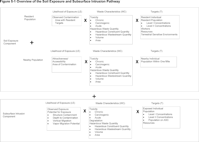
5.1 Soil exposure component. Evaluate the soil exposure component based on two threats: Resident population threat and nearby population threat. Evaluate both threats based on three factor categories: Likelihood of exposure, waste characteristics, and targets. Figure 5-1 indicates the factors included within each factor category for each type of threat.
Determine the soil exposure component score (S se) in terms of the factor category values as follows:
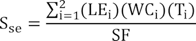
Where:
LE i = Likelihood of exposure factor category value for threat i (that is, resident population threat or nearby population threat).
WC i = Waste characteristics factor category value for threat i.
T i = Targets factor category value for threat i.
SF = Scaling factor.
Table 5-1 outlines the specific calculation procedure.
| Factor categories and factors | Maximum value | Value assigned |
|---|---|---|
| Resident Population Threat | ||
| Likelihood of Exposure: | ||
| 1. Likelihood of Exposure | 550 | |
| Waste Characteristics: | ||
| 2. Toxicity | (a) | |
| 3. Hazardous Waste Quantity | (a) | |
| 4. Waste Characteristics | 100 | |
| Targets: | ||
| 5. Resident Individual | 50 | |
| 6. Resident Population: | ||
| 6a. Level I Concentrations | (b) | |
| 6b. Level II Concentrations | (b) | |
| 6c. Resident Population (lines 6a + 6b) | (b) | |
| 7. Workers | 15 | |
| 8. Resources | 5 | |
| 9. Terrestrial Sensitive Environments | (c) | |
| 10. Targets (lines 5 + 6c + 7 + 8 + 9) | (b) | |
| Resident Population Threat Score: | ||
| 11. Resident Population Threat (lines 1 × 4 × 10) | (b) | |
| Nearby Population Threat | ||
| Likelihood of Exposure: | ||
| 12. Attractiveness/Accessibility | 100 | |
| 13. Area of Contamination | 100 | |
| 14. Likelihood of Exposure | 500 | |
| Waste Characteristics: | ||
| 15. Toxicity | (a) | |
| 16. Hazardous Waste Quantity | (a) | |
| 17. Waste Characteristics | 100 | |
| Targets: | ||
| 18. Nearby Individual | 1 | |
| 19. Population Within 1 Mile | (b) | |
| 20. Targets (lines 18 + 19) | (b) | |
| Nearby Population Threat Score: | ||
| 21. Nearby Population Threat (lines 14 × 17 × 20) | (b) | |
| Soil Exposure Component Score: | ||
| 22. Soil Exposure Component Score d (S se), (lines [11 + 21]/82,500, subject to a maximum of 100) | 100 | |
| a
Maximum value applies to waste characteristics category.
b Maximum value not applicable. c No specific maximum value applies to factor. However, pathway score based solely on terrestrial sensitive environments is limited to maximum of 60. d Do not round to nearest integer. | ||
5.1.0 General considerations. Evaluate the soil exposure component based on areas of observed contamination:
-
Consider observed contamination to be present at sampling locations where analytic evidence indicates that:
- —A hazardous substance attributable to the site is present at a concentration significantly above background levels for the site (see Table 2-3 in section 2.3 for the criteria for determining analytical significance), and
- —This hazardous substance, if not present at the surface, is covered by 2 feet or less of cover material (for example, soil).
-
Establish areas of observed contamination based on sampling locations at which there is observed contamination as follows:
- —For all sources except contaminated soil, if observed contamination from the site is present at any sampling location within the source, consider that entire source to be an area of observed contamination.
- —For contaminated soil, consider both the sampling location(s) with observed contamination from the site and the area lying between such locations to be an area of observed contamination, unless available information indicates otherwise.
- If an area of observed contamination (or portion of such an area) is covered by a permanent, or otherwise maintained, essentially impenetrable material (for example, asphalt) that is not more than 2 feet thick, exclude that area (or portion of the area) in evaluating the soil exposure component.
- For an area of observed contamination, consider only those hazardous substances that meet the criteria for observed contamination for that area to be associated with that area in evaluating the soil exposure component (see section 2.2.2).
If there is observed contamination, assign scores for the resident population threat and the nearby population threat, as specified in sections 5.1.1 and 5.1.2. If there is no observed contamination, assign the soil exposure component of the soil exposure and subsurface intrusion pathway a score of 0.
5.1.1 Resident population threat. Evaluate the resident population threat only if there is an area of observed contamination in one or more of the following locations:
- Within the property boundary of a residence, school, or day care center and within 200 feet of the respective residence, school, or day care center, or
- Within a workplace property boundary and within 200 feet of a workplace area, or
- Within the boundaries of a resource specified in section 5.1.1.3.4, or
- Within the boundaries of a terrestrial sensitive environment specified in section 5.1.1.3.5.
If not, assign the resident population threat a value of 0, enter this value in Table 5-1, and proceed to the nearby population threat (section 5.1.2).
5.1.1.1 Likelihood of exposure. Assign a value of 550 to the likelihood of exposure factor category for the resident population threat if there is an area of observed contamination in one or more locations listed in section 5.1.1. Enter this value in Table 5-1.
5.1.1.2 Waste characteristics. Evaluate waste characteristics based on two factors: toxicity and hazardous waste quantity. Evaluate only those hazardous substances that meet the criteria for observed contamination at the site (see section 5.1.0).
5.1.1.2.1 Toxicity. Assign a toxicity factor value to each hazardous substance as specified in section 2.4.1.1. Use the hazardous substance with the highest toxicity factor value to assign the value to the toxicity factor for the resident population threat. Enter this value in Table 5-1.
5.1.1.2.2 Hazardous waste quantity. Assign a hazardous waste quantity factor value as specified in section 2.4.2. In estimating the hazardous waste quantity, use Table 5-2 and:
- Consider only the first 2 feet of depth of an area of observed contamination, except as specified for the volume measure.
- Use the volume measure (see section 2.4.2.1.3) only for those types of areas of observed contamination listed in Tier C of Table 5-2. In evaluating the volume measure for these listed areas of observed contamination, use the full volume, not just the volume within the top 2 feet.
- Use the area measure (see section 2.4.2.1.4), not the volume measure, for all other types of areas of observed contamination, even if their volume is known.
Enter the value assigned in Table 5-1.
| Tier | Measure | Units | Equation for assigning value a |
|---|---|---|---|
| A | Hazardous Constituent Quantity (C) | lb | C. |
| B b | Hazardous Wastestream Quantity (W) | lb | W/5,000. |
| C b | Volume (V) Surface Impoundment c Drums d Tanks and Containers Other Than Drums |
yd
3 gallon yd 3 | V/2.5. V/500. V/2.5. |
| D b | Area (A) Landfill Surface Impoundment Surface Impoundment (Buried/backfilled) Land treatment Pile e Contaminated Soil |
ft
2 ft 2 ft 2 ft 2 ft 2 ft 2 | A/34,000. A/13. A/13. A/270. A/34. A/34,000. |
| a
Do not round nearest integer.
b Convert volume to mass when necessary: 1 ton = 2,000 pounds = 1 cubic yard = 4 drums = 200 gallons. c Use volume measure only for surface impoundments containing hazardous substances present as liquids. Use area measures in Tier D for dry surface impoundments and for buried/backfilled surface impoundments. d If actual volume of drums is unavailable, assume 1 drum = 50 gallons. e Use land surface area under pile, not surface area of pile. | |||
5.1.1.2.3 Calculation of waste characteristics factor category value. Multiply the toxicity and hazardous waste quantity factor values, subject to a maximum product of 1 × 10 8. Based on this product, assign a value from Table 2-7 (section 2.4.3.1) to the waste characteristics factor category. Enter this value in Table 5-1.
5.1.1.3 Targets. Evaluate the targets factor category for the resident population threat based on five factors: Resident individual, resident population, workers, resources, and terrestrial sensitive environments.
In evaluating the targets factor category for the resident population threat, count only the following as targets:
- Resident individual—a person living or attending school or day care on a property with an area of observed contamination and whose residence, school, or day care center, respectively, is on or within 200 feet of the area of observed contamination.
- Worker—a person working on a property with an area of observed contamination and whose workplace area is on or within 200 feet of the area of observed contamination.
- Resources located on an area of observed contamination, as specified in section 5.1.1.
- Terrestrial sensitive environments located on an area of observed contamination, as specified in section 5.1.1.
5.1.1.3.1 Resident individual. Evaluate this factor based on whether there is a resident individual, as specified in section 5.1.1.3, who is subject to Level I or Level II concentrations.
First, determine those areas of observed contamination subject to Level I concentrations and those subject to Level II concentrations as specified in sections 2.5.1 and 2.5.2. Use the health-based benchmarks from Table 5-3 in determining the level of contamination. Then assign a value to the resident individual factor as follows:
- Assign a value of 50 if there is at least one resident individual for one or more areas subject to Level I concentrations.
- Assign a value of 45 if there is no such resident individuals, but there is at least one resident individual for one or more areas subject to Level II concentrations.
- Assign a value of 0 if there is no resident individual.
Enter the value assigned in Table 5-1.
5.1.1.3.2 Resident population. Evaluate resident population based on two factors: Level I concentrations and Level II concentrations. Determine which factor applies as specified in sections 2.5.1 and 2.5.2, using the health-based benchmarks from Table 5-3. Evaluate populations subject to Level I concentrations as specified in section 5.1.1.3.2.1 and populations subject to Level II concentrations as specified in section 5.1.1.3.2.2.
| Screening concentration for cancer corresponding to that concentration that corresponds to the 10 −6 individual cancer risk for oral exposures. |
| Screening concentration for noncancer toxicological responses corresponding to the Reference Dose (RfD) for oral exposures. |
Count only those persons meeting the criteria for resident individual as specified in section 5.1.1.3. In estimating the number of people living on property with an area of observed contamination, when the estimate is based on the number of residences, multiply each residence by the average number of persons per residence for the county in which the residence is located.
5.1.1.3.2.1 Level I concentrations. Sum the number of resident individuals subject to Level I concentrations and multiply this sum by 10. Assign the resulting product as the value for this factor. Enter this value in Table 5-1.
5.1.1.3.2.2 Level II concentrations. Sum the number of resident individuals subject to Level II concentrations. Do not include those people already counted under the Level I concentrations factor. Assign this sum as the value for this factor. Enter this value in Table 5-1.
5.1.1.3.2.3 Calculation of resident population factor value. Sum the factor values for Level I concentrations and Level II concentrations. Assign this sum as the resident population factor value. Enter this value in Table 5-1.
5.1.1.3.3 Workers. Evaluate this factor based on the number of workers that meet the section 5.1.1.3 criteria. Assign a value for these workers using Table 5-4. Enter this value in Table 5-1.
| Number of workers | Assigned value |
|---|---|
| 0 | 0 |
| 1 to 100 | 5 |
| 101 to 1,000 | 10 |
| Greater than 1,000 | 15 |
5.1.1.3.4 Resources. Evaluate the resources factor as follows:
-
Assign a value of 5 to the resources factor if one or more of the following is present on an area of observed contamination at the site:
- —Commercial agriculture.
- —Commercial silviculture.
- —Commercial livestock production or commercial livestock grazing.
- Assign a value of 0 if none of the above are present.
Enter the value assigned in Table 5-1.
5.1.1.3.5 Terrestrial sensitive environments. Assign value(s) from Table 5-5 to each terrestrial sensitive environment that meets the eligibility criteria of section 5.1.1.3.
Calculate a value (ES) for terrestrial sensitive environments as follows:
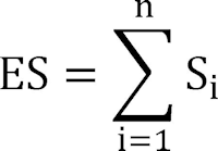
Where:
S i = Value(s) assigned from Table 5-5 to terrestrial sensitive environment i.
n = Number of terrestrial sensitive environments meeting section 5.1.1.3 criteria.
Because the pathway score based solely on terrestrial sensitive environments is limited to a maximum of 60, determine the value for the terrestrial sensitive environments factor as follows:
| Terrestrial sensitive environments | Assigned value |
|---|---|
| Terrestrial critical habitat a for Federal designated endangered or threatened species | 100 |
| National Park Designated Federal Wilderness Area National Monument | |
| Terrestrial habitat known to be used by Federal designated or proposed threatened or endangered species | 75 |
| National Preserve (terrestrial) National or State Terrestrial Wildlife Refuge Federal land designated for protection of natural ecosystems Administratively proposed Federal Wilderness Area Terrestrial areas utilized for breeding by large or dense aggregations of animals b | |
| Terrestrial habitat known to be used by State designated endangered or threatened species | 50 |
| Terrestrial habitat known to be used by species under review as to its Federal designated endangered or threatened status | |
| State lands designated for wildlife or game management | 25 |
| State designated Natural Areas Particular areas, relatively small in size, important to maintenance of unique biotic communities | |
| a
Critical habitat as defined in 50 CFR 424.02.
b Limit to vertebrate species. | |
-
Multiply the values assigned to the resident population threat for likelihood of exposure (LE), waste characteristics (WC), and ES. Divide the product by 82,500.
- —If the result is 60 or less, assign the value ES as the terrestrial sensitive environments factor value.
- —If the result exceeds 60, calculate a value EC as follows:
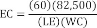
Assign the value EC as the terrestrial sensitive environments factor value. Do not round this value to the nearest integer.
Enter the value assigned for the terrestrial sensitive environments factor in Table 5-1.
5.1.1.3.6 Calculation of resident population targets factor category value. Sum the values for the resident individual, resident population, workers, resources, and terrestrial sensitive environments factors. Do not round to the nearest integer. Assign this sum as the targets factor category value for the resident population threat. Enter this value in Table 5-1.
5.1.1.4 Calculation of resident population threat score. Multiply the values for likelihood of exposure, waste characteristics, and targets for the resident population threat, and round the product to the nearest integer. Assign this product as the resident population threat score. Enter this score in Table 5-1.
5.1.2 Nearby population threat. Include in the nearby population only those individuals who live or attend school within a 1-mile travel distance of an area of observed contamination at the site and who do not meet the criteria for resident individual as specified in section 5.1.1.3.
Do not consider areas of observed contamination that have an attractiveness/accessibility factor value of 0 (see section 5.1.2.1.1) in evaluating the nearby population threat.
5.1.2.1 Likelihood of exposure. Evaluate two factors for the likelihood of exposure factor category for the nearby population threat: attractiveness/accessibility and area of contamination.
5.1.2.1.1 Attractiveness/accessibility. Assign a value for attractiveness/accessibility from Table 5-6 to each area of observed contamination, excluding any land used for residences. Select the highest value assigned to the areas evaluated and use it as the value for the attractiveness/accessibility factor. Enter this value in Table 5-1.
5.1.2.1.2 Area of contamination. Evaluate area of contamination based on the total area of the areas of observed contamination at the site. Count only the area(s) that meet the criteria in section 5.1.0 and that receive an attractiveness/accessibility value greater than 0. Assign a value to this factor from Table5-7. Enter this value in Table 5-1.
| Area of observed contamination | Assigned value |
|---|---|
| Designated recreational area | 100 |
| Regularly used for public recreation (for example, fishing, hiking, softball) | 75 |
| Accessible and unique recreational area (for example, vacant lots in urban area) | 75 |
| Moderately accessible (may have some access improvements, for example, gravel road), with some public recreation use | 50 |
| Slightly accessible (for example, extremely rural area with no road improvement), with some public recreation use | 25 |
| Accessible, with no public recreation use | 10 |
| Surrounded by maintained fence or combination of maintained fence and natural barriers | 5 |
| Physically inaccessible to public, with no evidence of public recreation use | 0 |
| Total area of the areas of observed contamination (square feet) | Assigned value |
|---|---|
| Less than or equal to 5,000 | 5 |
| Greater than 5,000 to 125,000 | 20 |
| Greater than 125,000 to 250,000 | 40 |
| Greater than 250,000 to 375,000 | 60 |
| Greater than 375,000 to 500,000 | 80 |
| Greater than 500,000 | 100 |
5.1.2.1.3 Likelihood of exposure factor category value. Assign a value from Table 5-8 to the likelihood of exposure factor category, based on the values assigned to the attractiveness/accessibility and area of contamination factors. Enter this value in Table 5-1.
| Area of contamination factor value | Attractiveness/accessibility factor value | ||||||
| 100 | 75 | 50 | 25 | 10 | 5 | 0 | |
| 100 | 500 | 500 | 375 | 250 | 125 | 50 | 0 |
| 80 | 500 | 375 | 250 | 125 | 50 | 25 | 0 |
| 60 | 375 | 250 | 125 | 50 | 25 | 5 | 0 |
| 40 | 250 | 125 | 50 | 25 | 5 | 5 | 0 |
| 20 | 125 | 50 | 25 | 5 | 5 | 5 | 0 |
| 5 | 50 | 25 | 5 | 5 | 5 | 5 | 0 |
5.1.2.2 Waste characteristics. Evaluate waste characteristics based on two factors: toxicity and hazardous waste quantity. Evaluate only those hazardous substances that meet the criteria for observed contamination (see section 5.1.0) at areas that can be assigned an attractiveness/accessibility factor value greater than 0.
5.1.2.2.1 Toxicity. Assign a toxicity factor value as specified in section 2.4.1.1 to each hazardous substance meeting the criteria in section 5.1.2.2. Use the hazardous substance with the highest toxicity factor value to assign the value to the toxicity factor for the nearby population threat. Enter this value in Table 5-1.
5.1.2.2.2 Hazardous waste quantity. Assign a value to the hazardous waste quantity factor as specified in section 5.1.1.2.2, except: consider only those areas of observed contamination that can be assigned an attractiveness/accessibility factor value greater than 0. Enter the value assigned in Table 5-1.
5.1.2.2.3 Calculation of waste characteristics factor category value. Multiply the toxicity and hazardous waste quantity factor values, subject to a maximum product of 1 × 10 8. Based on this product, assign a value from Table 2-7 (section 2.4.3.1) to the waste characteristics factor category. Enter this value in Table 5-1.
5.1.2.3 Targets. Evaluate the targets factory category for the nearby population threat based on two factors: nearby individual and population within a 1-mile travel distance from the site.
5.1.2.3.1 Nearby individual. If one or more persons meet the section 5.1.1.3 criteria for a resident individual, assign this factor a value of 0. Enter this value in Table 5-1.
If no person meets the criteria for a resident individual, determine the shortest travel distance from the site to any residence or school. In determining the travel distance, measure the shortest overland distance an individual would travel from a residence or school to the nearest area of observed contamination for the site with an attractiveness/accessibility factor value greater than 0. If there are no natural barriers to travel, measure the travel distance as the shortest straight-line distance from the residence or school to the area of observed contamination. If natural barriers exist (for example, a river), measure the travel distance as the shortest straight-line distance from the residence or school to the nearest crossing point and from there as the shortest straight- line distance to the area of observed contamination. Based on the shortest travel distance, assign a value from Table 5-9 to the nearest individual factor. Enter this value in Table 5-1.
| Travel distance for nearby individual (miles) | Assigned value |
|---|---|
| Greater than 0 to 1/4 | a 1 |
| Greater than 1/4 to 1 | 0 |
| a Assign a value of 0 if one or more persons meet the section 5.1.1.3 criteria for resident individual. | |
5.1.2.3.2 Population within 1 mile. Determine the population within each travel distance category of Table 5-10. Count residents and students who attend school within this travel distance. Do not include those people already counted in the resident population threat. Determine travel distances as specified in section 5.1.2.3.1.
In estimating residential population, when the estimate is based on the number of residences, multiply each residence by the average number of persons per residence for the county in which the residence is located.
Based on the number of people included within a travel distance category, assign a distance-weighted population value for that travel distance from Table 5-10.
Calculate the value for the population within 1 mile factor (PN) as follows:
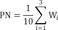
Where:
W i =Distance-weighted population value from Table 5-10 for travel distance category i.
If PN is less than 1, do not round it to the nearest integer; if PN is 1 or more, round to the nearest integer. Enter this value in Table 5-1.
5.1.2.3.3 Calculation of nearby population targets factor category value. Sum the values for the nearby individual factor and the population within 1 mile factor. Do not round this sum to the nearest integer. Assign this sum as the targets factor category value for the nearby population threat. Enter this value in Table 5-1.
| Travel distance category (miles) | Number of people within the travel distance category | |||||||||||
| 0 | 1 to 10 | 11 to 30 | 31 to 100 | 101 to 300 | 301 to 1,000 | 1,001 to 3,000 | 3,001 to 10,000 | 10,001 to 30,000 | 30,001 to 100,000 | 100,001 to 300,000 | 300,001 to 1,000,000 | |
| Greater than 0 to 1/4 | 0 | 0.1 | 0.4 | 1.0 | 4 | 13 | 41 | 130 | 408 | 1,303 | 4,081 | 13,034 |
| Greater than 1/4 to 1/2 | 0 | 0.05 | 0.2 | 0.7 | 2 | 7 | 20 | 65 | 204 | 652 | 2,041 | 6,517 |
| Greater than 1/2 to 1 | 0 | 0.02 | 0.1 | 0.3 | 1 | 3 | 10 | 33 | 102 | 326 | 1,020 | 3,258 |
| a Round the number of people present within a travel distance category to nearest integer. Do not round the assigned distance-weighted population value to nearest integer. | ||||||||||||
5.1.2.4 Calculation of nearby population threat score. Multiply the values for likelihood of exposure, waste characteristics, and targets for the nearby population threat, and round the product to the nearest integer. Assign this product as the nearby population threat score. Enter this score in Table 5-1.
5.1.3 Calculation of soil exposure component score. Sum the resident population threat score and the nearby population threat score, and divide the sum by 82,500. Assign the resulting value, subject to a maximum of 100, as the soil exposure component score (S se). Enter this score in Table 5-1.
5.2 Subsurface intrusion component. Evaluate the subsurface intrusion component based on three factor categories: likelihood of exposure, waste characteristics, and targets. Figure 5-1 indicates the factors included within each factor category for the subsurface intrusion component.
Determine the component score (S ssi) in terms of the factor category values as follows:
Where:
LE=Likelihood of exposure factor category value.
WC=Waste characteristics factor category value.
T=Targets factor category value.
SF=Scaling factor.
Table 5-11 outlines the specific calculation procedure.
| Factor categories and factors | Maximum value | Value assigned |
|---|---|---|
| Subsurface Intrusion Component: | ||
| Likelihood of Exposure: | ||
| 1. Observed Exposure | 550 | |
| 2. Potential for Exposure | ||
| 2a. Structure Containment | 10 | |
| 2b. Depth to contamination | 10 | |
| 2c. Vertical Migration | 15 | |
| 2d. Vapor Migration Potential | 25 | |
| 3. Potential for Exposure (lines 2a * (2b + 2c + 2d), subject to a maximum of 500) | 500 | |
| 4. Likelihood of Exposure (higher of lines 1 or 3) | 550 | |
| Waste Characteristics: | ||
| 5. Toxicity/Degradation | (a) | |
| 6. Hazardous Waste Quantity | (a) | |
| 7. Waste Characteristics (subject to a maximum of 100) | 100 | |
| Targets: | ||
| 8. Exposed Individual | 50 | |
| 9. Population: | ||
| 9a. Level I Concentrations | (b) | |
| 9b. Level II Concentrations | (b) | |
| 9c. Population within an Area of Subsurface Contamination | (b) | |
| 9d. Total Population (lines 9a + 9b + 9c) | (b) | |
| 10. Resources | 5 | |
| 11. Targets (lines 8 + 9d + 10) | (b) | |
| Subsurface Intrusion Component Score: | ||
| 12. Subsurface Intrusion Component (lines 4 × 7 × 11)/82,500 c (subject to a maximum of 100) | 100 | |
| Soil Exposure and Subsurface Intrusion Pathway Score: | ||
| 13. Soil Exposure Component + Subsurface Intrusion Component (subject to a maximum of 100) | 100 | |
| a
Maximum value applies to waste characteristics category.
b Maximum value not applicable. c Do not round to the nearest integer. | ||
5.2.0 General considerations. The subsurface intrusion component evaluates the threats from hazardous substances that have or could intrude into regularly occupied structures from the subsurface. Evaluate the subsurface intrusion component based on the actual or potential intrusion of hazardous substances into all regularly occupied structures that have structure containment values greater than zero and meet the criteria identified in the section below as being either in an area of observed exposure or in an area of subsurface contamination. These structures may or may not have subunits. Subunits are partitioned areas within a structure with separate heating, ventilating, and air conditioning (HVAC) systems or distinctly different air exchange rates. Subunits include regularly occupied partitioned tenant spaces such as office suites, apartments, condos, common or shared areas, and portions of residential, commercial or industrial structures with separate heating, ventilating, and air conditioning (HVAC) systems.
In evaluating the subsurface intrusion component, consider the following:
-
Area(s) of observed exposure: An area of observed exposure is delineated by regularly occupied structures with documented contamination meeting observed exposure criteria; an area of observed exposure includes regularly occupied structures with samples meeting observed exposure criteria or inferred to be within an area of observed exposure based on samples meeting observed exposure criteria (see section 5.2.1.1.1
Observed exposure). Establish areas of observed exposure as follows:
- —For regularly occupied structures that have no subunits, consider both the regularly occupied structures containing sampling location(s) meeting observed exposure criteria for the site and the regularly occupied structure(s) in the area lying between such locations to be an area of observed exposure (i.e., inferred to be in an area of observed exposure), unless available information indicates otherwise.
- —In multi-story, multi-subunit, regularly occupied structures, consider all subunits on a level with sampling locations meeting observed exposure criteria from the site and all levels below, if any, to be within an area of observed exposure, unless available information indicates otherwise.
- —In multi-tenant structures, that do not have a documented observed exposure, but are located in an area lying between locations where observed exposures have been documented, consider only those regularly occupied subunits, if any, on the lowest level of the structure, to be within an area of observed exposure (i.e., inferred to be in an area of observed exposure, unless available information indicates otherwise.
-
Area(s) of subsurface contamination: An area of subsurface contamination is delineated by sampling
locations meeting observed release criteria for subsurface intrusion, excluding areas of observed exposure
(see Table 2-3 in section 2.3). The area within an area of subsurface contamination includes potentially
exposed populations. If the significant increase in hazardous substance levels cannot be attributed at
least in part to the site, and cannot be attributed to other sites, attribution can be established based
on the presence of hazardous substances in the area of subsurface contamination. Establish areas of subsurface
contamination as follows:
- —Exclude those areas that contain structures meeting the criteria defined as an area of observed exposure.
-
—Consider both the sampling location(s) with subsurface contamination meeting observed release criteria from the site and the area lying between such locations to be an area of subsurface contamination (i.e.,
inferred to be in an area of subsurface contamination). If sufficient data is available and state of the science shows there is no unacceptable risk due to subsurface intrusion into a regularly occupied structure located within an area of subsurface contamination, that structure can be excluded from the area of subsurface contamination.
Evaluate an area of subsurface contamination based on hazardous substances that:- Meet the criteria for observed exposure of a chemical that has a vapor pressure greater than or equal to one torr or a Henry's constant greater than or equal to 10 −5 atm-m 3 /mol, or
- Meet the criteria for observed release in an area of subsurface contamination and have a vapor pressure greater than or equal to one torr or a Henry's constant greater than or equal to 10 −5 atm-m 3 /mol, or
- Meet the criteria for an observed release in a structure within, or in a sample from below, an area of observed exposure and have a vapor pressure greater than or equal to one torr or a Henry's constant greater than or equal to 10 −5 atm-m 3 /mol.
- —Evaluate all structures with no subunits that have containment factor values greater than zero, and not documented to meet observed exposure criteria to be in an area of subsurface contamination if they are lying between locations of subsurface intrusion samples meeting observed release criteria.
-
—Evaluate multi-subunit structures as follows:
- If an observed exposure has been documented based on a gaseous indoor air sample, consider all regularly occupied subunit(s), if any, on the level immediately above the level where an observed exposure has been documented (or has been inferred to be within an area of observed exposure), to be within an area of subsurface contamination. If sufficient data is available and state of the science shows there is no unacceptable risk due to subsurface intrusion on the level immediately above the level where an observed exposure has been documented (or has been inferred to be within an area of observed exposure) that level can be excluded from the area of subsurface contamination.
- If observed release criteria have been met based on a gaseous indoor air sample collected from a level not regularly occupied, consider all regularly occupied subunit(s), if any, on the level immediately above the level where the observed release criteria has been documented, to be within an area of subsurface contamination. If sufficient data is available and state of the science shows there is no unacceptable risk due to subsurface intrusion on the level immediately above the level where the observed release criteria has been documented that level can be excluded from the area of subsurface contamination.
- If any regularly occupied multi-subunit structure is inferred to be in an area of subsurface contamination, consider only those regularly occupied subunit(s), if any, on the lowest level, to be within an area of subsurface contamination. If sufficient data is available and state of the science shows there is no unacceptable risk due to subsurface intrusion on the lowest level, that structure can be excluded from the area of subsurface contamination.
See Section 7.0 for establishing an area of subsurface contamination based on the presence of radioactive hazardous substances.
If there is no area of observed exposure and no area of subsurface contamination, assign a score of 0 for the subsurface intrusion component.
5.2.1 Subsurface intrusion component. Evaluate this component only if there is an area of observed exposure or area of subsurface contamination:
- Within or underlying a residence, school, day care center, workplace, or
- Within or underlying a resource specified in section 5.2.1.3.3.
5.2.1.1 Likelihood of exposure. Assign a value of 550 to the likelihood of exposure factor category for the subsurface intrusion component if there is an area of observed exposure in one or more locations listed in section 5.2.1. Enter this value in Table 5-11.
5.2.1.1.1 Observed exposure. Establish observed exposure in a regularly occupied structure by demonstrating that a hazardous substance has been released into a regularly occupied structure via the subsurface. Base this demonstration on either of the following criteria:
-
Direct observation:
- —A solid, liquid, or gaseous material that contains one or more hazardous substances attributable to the site has been observed entering a regularly occupied structure through migration via the subsurface or is known to have entered a regularly occupied structure via the subsurface, or
- —When evidence supports the inference of subsurface intrusion of a material that contains one or more hazardous substances associated with the site into a regularly occupied structure, demonstrated adverse effects associated with that release may be used to establish observed exposure.
-
Chemical analysis:
- —Analysis of indoor samples indicates that the concentration of hazardous substance(s) is significantly above the background concentration for the site for that type of sample (see section 2.3).
- —Some portion of the significant increase above background must be attributable to the site to establish the observed exposure. Documentation of this attribution should account for possible concentrations of the hazardous substance(s) in outdoor air or from materials found in the regularly occupied structure, and should provide a rationale for the increase being from subsurface intrusion.
If observed exposure can be established in a regularly occupied structure, assign an observed exposure factor value of 550, enter this value in Table 5-11, and proceed to section 5.2.1.1.3. If no observed exposure can be established, assign an observed exposure factor value of 0, enter this value in Table 5-11, and proceed to section 5.2.1.1.2.
5.2.1.1.2 Potential for exposure. Evaluate potential for exposure only if an observed exposure cannot be established, but an area of subsurface contamination has been delineated. Evaluate potential for exposure based only on the presence of hazardous substances with a vapor pressure greater than or equal to one torr or a Henry's constant greater than or equal to 10 −5 atm-m 3 /mol. Evaluate potential for exposure for each area of subsurface contamination based on four factors: Structure containment (see section 5.2.1.1.2.1), depth to contamination (see section 5.2.1.1.2.2), vertical migration (see section 5.2.1.1.2.3) and vapor migration potential (see section 5.2.1.1.2.4). For each area of subsurface contamination, assign the highest value for each factor. If information is insufficient to calculate any single factor value used to calculate the potential for exposure factor values at an identified area of subsurface contamination, information collected for another area of subsurface contamination at the site may be used when evaluating potential for exposure. Calculate the potential for exposure value for the site as specified in section 5.2.1.1.2.5.
5.2.1.1.2.1 Structure containment. Calculate containment for eligible hazardous substances within this component as directed in Table 5-12 and enter this value into Table 5-11. Assign each regularly occupied structure within an area of subsurface contamination the highest appropriate structure containment value from Table 5-12 and use the regularly occupied structure at the site with the highest structure containment value in performing the potential for exposure calculation. For all regularly occupied structures with unknown containment features assign a structure containment value of greater than zero for the purposes of evaluating targets (see section 5.2.1.3).
| No. | Evidence of structure containment | Assigned value |
|---|---|---|
| 1. | Regularly occupied structure with evidence of subsurface intrusion, including documented observed exposure or sampling of bio or inert gases, such as methane and radon | 10 |
| 2. | Regularly occupied structure with open preferential subsurface intrusion pathways (e.g., sumps, foundation cracks, unsealed utility lines) | 10 |
| 3. | Regularly occupied structure with an engineered vapor migration barrier system that does not address all preferential subsurface intrusion pathways | 7 |
| 4. | Regularly occupied structure with an engineered passive vapor mitigation system without documented institutional controls (e.g., deed restrictions) or evidence of regular maintenance and inspection | 6 |
| 5. | Regularly occupied structure with no visible open preferential subsurface intrusion pathways from the subsurface (e.g., sumps, foundation cracks, unsealed utility lines) | 4 |
| 6. | Regularly occupied structure with an engineered passive vapor mitigation system (e.g., passive venting) with documented institutional controls (e.g., deed restrictions) or evidence of regular maintenance and inspection | 3 |
| 7. | Regularly occupied structure with an engineered, active vapor mitigation system (e.g., active venting) without documented institutional controls (e.g., deed restrictions) and funding in place for on-going operation, inspection and maintenance | 2 |
| 8. | Regularly occupied structure with a permanent engineered, active vapor mitigation system (e.g., active venting) with documented institutional controls (e.g., deed restrictions) and funding in place for on-going operation, inspection and maintenance | 1 |
| 9. | Regularly occupied structure with a foundation raised greater than 6 feet above ground surface (e.g., structure on stilts) or structure that has been built, and maintained, in a manner to prevent subsurface intrusion | 0 |
5.2.1.1.2.2 Depth to contamination. Assign each area of subsurface contamination a depth to contamination based on the least depth to either contaminated crawl space or subsurface media underlying a regularly occupied structure. Measure this depth to contamination based on the distance between the lowest point of a regularly occupied structure to the highest known point of hazardous substances eligible to be evaluated. Use any regularly occupied structure within an area of subsurface contamination with a structure containment factor value greater than zero. Subtract from the depth to contamination the thickness of any subsurface layer composed of features that would allow channelized flow (e.g., karst, lava tubes, open fractures, as well as manmade preferential pathways such as utility conduits or drainage systems).
Based on this calculated depth, assign a factor value from Table 5-13. If the necessary information is available at multiple locations, calculate the depth to contamination at each location. Use the location having the least depth to contamination to assign the factor value. Enter this value in Table 5-11.
| Depth range | Depth to contamination assigned value |
|---|---|
| 0 to <10 ft (Including subslab and semi-enclosed or enclosed crawl space contamination) | 10 |
| >10 to 20 ft | 8 |
| >20 to 50 ft | 6 |
| >50 to 100 ft | 4 |
| >100 to 150 ft | 2 |
| >150 ft | 0 |
| 1 If any part of the subsurface profile has channelized flow features, assign that portion of the subsurface profile a depth of 0. | |
| 2 Measure elevation below any regularly occupied structure within an area of subsurface contamination at a site. Select the regularly occupied structure with the least depth to contamination below a structure. | |
5.2.1.1.2.3 Vertical migration. Evaluate the vertical migration factor for each area of subsurface contamination based on the geologic materials in the interval between the lowest point of a regularly occupied structure and the highest known point of hazardous substances in the subsurface. Use any regularly occupied structure either within an area of subsurface contamination or overlying subsurface soil gas or ground water contamination. Assign a value to the vertical migration factor as follows:
- If the depth to contamination (see section 5.2.1.1.2.2) is 10 feet or less, assign a value of 15.
- If the depth to contamination is greater than 10 feet, do not consider layers or portions of layers within the first 10 feet of the depth to contamination (as assigned in section 5.2.1.1.2.2).
- If, for the interval between the lowest point of a regularly occupied structure and the highest point of hazardous substances in the subsurface, all layers that underlie a portion of a regularly occupied structure at the site are karst or otherwise allow channelized flow, assign a value of 15.
-
Otherwise:
- —Select the lowest effective porosity/permeability layer(s) from within the interval identified above. Consider only layers at least 1 foot thick.—Assign a value for individual layers from Table 5-14 using the hydraulic conductivity of the layer, if available. If the hydraulic conductivity is not available, assign a value based on the type of material in the selected layer.
- —If more than one layer has the same assigned porosity/permeability value, include all such layers and sum their thicknesses. Assign a thickness of 0 feet to a layer with channelized flow features found within any area of subsurface contamination at the site.
- —Assign a value from Table 5-15 to the vertical migration factor, based on the thickness and assigned porosity/permeability value of the lowest effective porosity/permeability layer(s).
Determine vertical migration only at locations within an area of subsurface contamination at the site. If the necessary subsurface geologic information is available at multiple locations, evaluate the vertical migration factor at each location. Use the location having the highest vertical migration factor value to assign the factor value. Enter this value in Table 5-11.
| Type of material | Hydraulic conductivity (cm/sec) | Assigned porosity/ permeability value |
|---|---|---|
| Gravel; clean sand; highly permeable fractured igneous and metamorphic rocks; permeable basalt; karst limestones and dolomites | Greater than or equal to 1 × 10 −3 | 1 |
| Sand; sandy clays; sandy loams; loamy sands; sandy silts; sediments that are predominantly sand; highly permeable till (coarse-grained, unconsolidated or compact and highly fractured); peat; moderately permeable limestones and dolomites (no karst); moderately permeable sandstone; moderately permeable fractured igneous and metamorphic rocks | Less than 1 × 10 −3 | 2 |
| Silt; loams; silty loams; loesses; silty clays; sediments that are predominantly silts; moderately permeable till (fine-grained, unconsolidated till, or compact till with some fractures); low permeability limestones and dolomites (no karst); low permeability sandstone; low permeability fractured igneous and metamorphic rocks | Less than 1 × 10 −5 | 3 |
| Clay; low permeability till (compact unfractured till); shale; unfractured metamorphic and igneous rocks | Less than 1 × 10 −7 | 4 |
| Assigned porosity/permeability value | Thickness of lowest porosity layer(s) b (feet) | |||||
| 0 to 5 | Greater than 5 to 10 | Greater than 10 to 20 | Greater than 20 to 50 | Greater than 50 to 100 | Greater than 100 to 150 | |
| 1 | 15 | 15 | 14 | 11 | 8 | 6 |
| 2 | 15 | 14 | 12 | 9 | 6 | 4 |
| 3 | 15 | 13 | 10 | 7 | 5 | 2 |
| 4 | 15 | 12 | 9 | 6 | 3 | 1 |
| a
If depth to contamination is 10 feet or less or if, for the interval being evaluated, all layers that underlie a portion of the structure at the site are karst or have other channelized flow features, assign a value of 15.
b Consider only layers at least 1 foot thick. | ||||||
5.2.1.1.2.4 Vapor migration potential. Evaluate this factor for each area of subsurface contamination as follows:
- If the depth to contamination (see section 5.2.1.1.2.2) is 10 feet or less, assign a value of 25.
-
Assign a value for vapor migration potential to each of the gaseous hazardous substances associated with the area of subsurface contamination (see section 2.2.2) as follows:
- —Assign values from Table 5-16 for both vapor pressure and Henry's constant to each hazardous substance. If Henry's constant cannot be determined for a hazardous substance, assign that hazardous substance a value of 2 for the Henry's constant component.
- —Sum the two values assigned to each hazardous substance.
- —Based on this sum, assign each hazardous substance a value from Table 5-17 for vapor migration potential.
-
Assign a value for vapor migration potential to each area of subsurface contamination as follows:
- —Select the hazardous substance associated with the area of subsurface contamination with the highest vapor migration potential value and assign this value as the vapor migration potential factor value for the area of subsurface contamination.
Enter this value in Table 5-11.
| Assigned value | |
|---|---|
| Vapor Pressure (Torr): | |
| Greater than 10 | 3 |
| 1 to 10 | 2 |
| Less than 1 | 0 |
| Henry's Constant (atm-m 3 /mol): | |
| Greater than 10 −3 | 3 |
| Greater than 10 −4 to 10 −3 | 2 |
| 10 −5 to 10 −4 | 1 |
| Less than 10 −5 | 0 |
| Sum of values for vapor pressure and Henry's constant | Assigned value |
|---|---|
| 0 | 0 |
| 1 or 2 | 5 |
| 3 or 4 | 15 |
| 5 or 6 | 25 |
5.2.1.1.2.5 Calculation of potential for exposure factor value. For each identified area of subsurface contamination, sum the factor values for depth to contamination, vertical migration, and vapor migration potential, and multiply this sum by the factor value for structure containment. Select the highest product for any area of subsurface contamination and assign this value as the potential for exposure factor value for the component. Enter this value in Table 5-11.
5.2.1.1.3 Calculation of likelihood of exposure factor category value. If observed exposure is established for the site, assign the observed exposure factor value of 550 as the likelihood of exposure factor category value for the site. Otherwise, assign the potential for exposure factor value for the component as the likelihood of exposure value. Enter the value assigned in Table 5-11.
5.2.1.2 Waste characteristics. Evaluate waste characteristics based on two factors: toxicity/degradation and hazardous waste quantity.
5.2.1.2.1 Toxicity/degradation. For each hazardous substance, assign a toxicity factor value, a degradation factor value and a combined toxicity/degradation factor value as specified in sections 2.2.3, 2.4.1.2 and 5.2.1.2.1.1 through 5.2.1.2.1.3.
5.2.1.2.1.1 Toxicity. Assign a toxicity factor value to each hazardous substance as specified in sections 2.2.2 and 2.4.1.1.
5.2.1.2.1.2 Degradation. Assign a degradation factor value to each hazardous substance as follows:
- For any hazardous substance that meets the criteria for an observed exposure, or if a NAPL is present in the subsurface below an area of observed exposure or area of subsurface contamination at a depth less than or equal to 30 feet, assign that substance a degradation factor value of 1.
- For all other situations, assign a degradation factor value using Table 5-18. Assign the depth to contamination as directed in section 5.2.1.1.2.2, except if evidence indicates that biologically active soil is not present throughout the depth beneath any regularly occupied structure. In this situation, subtract any thickness of non-biologically active soil from the estimated depth to contamination.
| Depth to contamination (feet) a | Half-life | ||
| >100 Days | >30 days and ≤100 days | ≤30 days | |
| <10 | 1 | 1 | 1 |
| 10 to ≤30 | 1 | 1 | 0.1 |
| >30 | 1 | 0.5 | 0.1 |
| a When determining the depth to contamination do not include layers of non-biologically-active soil, nor subsurface intervals with channelized flow (e.g., karst, lava tubes, open fractures, and manmade preferential pathways as directed in section 5.2.1.1.2.2). | |||
Calculate the half-life for each hazardous substance that meets subsurface intrusion observed release criteria as follows:
The half-life of a substance in the subsurface is defined for HRS purposes as the time required to reduce the initial concentration of the substance in the subsurface by one-half as a result of the combined decay processes of two components: Biodegradation and hydrolysis.
Estimate the half-life (t 1/2) of a hazardous substance as follows:
Where:
h=Hydrolysis half-life.
b=Biodegradation half-life.
If either of these component half-lives cannot be estimated for the hazardous substance from available data, delete that component half-life from the above equation.
If no half-life information is available for a hazardous substance and the substance is not already assigned a value of 1, unless information indicates otherwise, assign a value of 1.
5.2.1.2.1.3 Calculation of toxicity/degradation factor value. Assign each substance a toxicity/degradation value by multiplying the toxicity factor value by the degradation factor value. Use the hazardous substance with the highest combined toxicity/degradation value to assign the factor value to the toxicity/degradation factor for the subsurface intrusion threat. Enter this value in Table 5-11.
5.2.1.2.2 Hazardous waste quantity. Assign a hazardous waste quantity factor value as specified in section 2.4.2. Consider only those regularly occupied structures or subunits with a non-zero structure containment value. Also include all regularly occupied structures or subunits that have had mitigation systems installed as part of a removal or other temporary response action. If sufficient structure-specific concentration data is available and state of the science shows there is no unacceptable risk of exposure to populations in a regularly occupied structure or subunit in an area of subsurface contamination, that structure or subunit is not included in the hazardous waste quantity evaluation. In estimating the hazardous waste quantity, use Tables 2-5 and 5-19 and:
-
For Tier A, hazardous constituent quantity, use the mass of constituents found in the regularly occupied structure(s) where the observed exposure has been identified.
- —For multi-subunit structures, when calculating Tier A, use the mass of constituents found in the regularly occupied subunit space(s) where the observed exposure has been identified.
-
For Tier B, hazardous wastestream quantity, use the flow-through volume of the regularly occupied structures where the observed exposure has been identified.
- —For multi-subunit structures, when calculating Tier B, use the flow-through volume of the regularly occupied subunit spaces where the observed exposure has been identified.
-
For Tier C, volume, use the volume divisor listed in Tier C of Table 5-19. Volume is calculated for those regularly occupied structures located within areas of observed exposure with observed or inferred intrusion and within areas of subsurface contamination.
-
—In evaluating the volume measure for these listed areas of observed exposure and areas of subsurface contamination based on a gaseous/vapor intrusion or the potential for gaseous/vapor intrusion, consider the following:
- Calculate the volume of each regularly occupied structure based on actual data. If unknown, use a ceiling height of 8 feet.
- For multi-subunit structures, when calculating Tier C, calculate volume for those subunit spaces with observed or inferred exposure and all other regularly occupied subunit spaces on that level, unless available information indicates otherwise. If the structure has multiple stories, also include the volume of all regularly occupied subunit spaces below the floor with an observed exposure and one story above, unless evidence indicates otherwise.
- For multi-subunit structures within an area of subsurface contamination and no observed or inferred exposure, consider only the volume of the regularly occupied subunit spaces on the lowest story, unless available information indicates otherwise.
- For Tier D, area, if volume is unknown, use the area divisor listed in Tier D of Table 5-19 for those regularly occupied structures within areas of observed exposure with observed or inferred intrusion and within areas of subsurface contamination.
-
—In evaluating the area measure for these listed areas of observed exposure and areas of subsurface contamination, calculate the area of each regularly occupied structure (including multi-subunit structures) or subunit based on actual footprint area data.
- If the actual footprint area of the structure(s) is unknown, use an area of 1,740 square feet for each structure (or subunit space).
- For multi-subunit structures, when calculating Tier D, calculate area for those subunit spaces with observed or inferred exposure and all other regularly occupied subunit spaces on that level, unless available information indicates otherwise. If the structure has multiple stories, also include the area of all regularly occupied subunit spaces below the floor with an observed exposure and one story above, unless evidence indicates otherwise.
- For multi-subunit structures within an area of subsurface contamination and no observed or inferred exposure, consider only the area of the regularly occupied subunit spaces on the lowest story, unless available information indicates otherwise.
-
—In evaluating the volume measure for these listed areas of observed exposure and areas of subsurface contamination based on a gaseous/vapor intrusion or the potential for gaseous/vapor intrusion, consider the following:
| Tier | Measure | Units | Equation for assigning value a |
|---|---|---|---|
| A | Hazardous Constituent Quantity (C) | Lb | C |
| B b | Hazardous Wastestream Quantity (W) | Lb | W/5,000 |
| C b,c | Volume (V) | ||
| Regularly occupied structure(s) in areas of observed exposure or subsurface contamination | yd 3 | V/2.5 | |
| D b,d | Area (A) | ||
| Regularly occupied structure(s) in areas of observed exposure or subsurface contamination | ft 2 | A/13 | |
| a
Do not round to the nearest integer.
b Convert volume to mass when necessary: 1 ton=2,000 pounds=1 cubic yard=4 drums=200 gallons. c Calculate volume of each regularly occupied structure or subunit space in areas of observed exposure and areas of subsurface contamination—Assume 8-foot ceiling height unless actual value is known. d Calculate area of the footprint of each regularly occupied structure in areas of observed exposure and areas of subsurface contamination. If the footprint area of a regularly occupied structure is unknown, use 1,740 square feet as the footprint area of the structure or subunit space. | |||
For the subsurface intrusion component, if the hazardous constituent quantity is adequately determined for all areas of observed exposure, assign the value from Table 2-6 as the hazardous waste quantity factor value. If the hazardous constituent quantity is not adequately determined for one or more areas of observed exposure or if one or more areas of subsurface contamination are present, assign either the value from Table 2-6 or assign a factor value as follows:
- If any target for the subsurface intrusion component is subject to Level I or Level II concentrations (see section 2.5), assign either the value from Table 2-6 or a value of 100, whichever is greater, as the hazardous waste quantity factor value for this component.
-
If none of the targets for the subsurface intrusion component is subject to Level I or Level II concentrations and if there has been a removal action that does not permanently interrupt target exposure from subsurface intrusion, and if an area of subsurface contamination exists, assign a factor value as follows:
- —Determine the values from Table 2-6 with and without consideration of the removal action.
- —If the value that would be assigned from Table 2-6 without consideration of the removal action would be 100 or greater, assign either the value from Table 2-6 with consideration of the removal action or a value of 100, whichever is greater, as the hazardous waste quantity factor value for the component.
- —If the value that would be assigned from Table 2-6 without consideration of the removal action would be less than 100, assign a value of 10 as the hazardous waste quantity factor value for the component.
- Otherwise, if none of the targets for the subsurface intrusion component is subject to Level I or Level II concentrations and there has not been a removal action, assign a value from Table 2-6 or a value of 10, whichever is greater.
Enter the value assigned in Table 5-11.
5.2.1.2.3 Calculation of waste characteristics factor category value. Multiply the toxicity/degradation and hazardous waste quantity factor values, subject to a maximum product of 1 × 10 8. Based on this product, assign a value from Table 2-7 (section 2.4.3.1) to the waste characteristics factor category. Enter this value in Table 5-11.
5.2.1.3 Targets. Evaluate the targets factor category for the subsurface intrusion threat based on three factors: Exposed individual, population, and resources in regularly occupied structures with structure containment factors greater than 0. Evaluate only those targets within areas of observed exposure and areas of subsurface contamination (see section 5.2.0).
In evaluating the targets factor category for the subsurface intrusion threat, count only the following as targets:
- Exposed individual—a person living, attending school or day care, or working in a regularly occupied structure with observed exposure or in a structure within an area of observed exposure or within an area of subsurface contamination.
- Population—exposed individuals in a regularly occupied structure within an area of observed exposure or within an area of subsurface contamination.
- Resources—located within an area of observed exposure or within an area of subsurface contamination as specified in section 5.2.1.3.3.
If a formerly occupied structure has been vacated due to subsurface intrusion attributable to the site, count the initial targets as if they were still residing in the structure. In addition, if a removal or temporary response action has occurred that has not completely mitigated the release, count the initial targets as if the removal or temporary response action has not permanently interrupted target exposure from subsurface intrusion. Evaluate those targets based on conditions at the time of removal of temporary response action.
For populations residing in or working in a multi-subunit structure with multiple stories in an area of observed exposure or area of subsurface contamination, count these targets as follows:
- If there is no observed exposure within the structure, include in the evaluation only those targets, if any, in the lowest occupied level. If sufficient structure-specific concentration data is available and state of the science shows there is no unacceptable risk of exposure to targets in the lowest level, those targets are not included in the evaluation.
- If there is an observed exposure in any level, include in the evaluation those targets in that level, the level above and all levels below. (The weighting of these targets is specified in Section 5.2.1.3.2.) If sufficient structure-specific concentration data is available and state of the science shows there is no unacceptable risk of exposure to targets in the level above where the observed exposure has been documented, those targets are not included in the evaluation.
5.2.1.3.1 Exposed individual. Evaluate this factor based on whether there is an exposed individual, as specified in sections 2.5.1, 2.5.2 and 5.2.1.3, who is subject to Level I or Level II concentrations.
First, determine those regularly occupied structures or partitioned subunit(s) within structures in an area of observed exposure subject to Level I concentrations and those subject to Level II concentrations as specified as follows (see section 5.2.0):
-
Level I Concentrations: For contamination resulting from subsurface intrusion, compare the hazardous substance concentrations in any sample meeting the observed exposure by chemical analysis criteria to the appropriate benchmark. Use the health-based benchmarks from Table 5-20 to determine the level of contamination.
- —If the sample is from a structure with no subunits and the concentration equals or exceeds the appropriate benchmark, assign Level I concentrations to the entire structure.
- —If the sample is from a subunit within a structure and the concentration from that subunit equals or exceeds the appropriate benchmark, assign Level I concentrations to that subunit.
-
Level II Concentrations: Structures, or subunits within structures, with one or more samples that meet observed exposure by chemical analysis criteria but do not equal or exceed the appropriate benchmark; structures, or subunits, that have an observed exposure by direct observation; and structures inferred to be in an area of observed exposure based on samples meeting observed exposure, are assigned Level II concentrations.
- —For all regularly occupied structures, or subunits in such structures, in an area of observed exposure that are not assigned Level I concentrations, assign Level II concentrations.
Then assign a value to the exposed individual factor as follows:
- Assign a value of 50 if there is at least one exposed individual in one or more regularly occupied structures subject to Level I concentrations.
- Assign a value of 45 if there are no Level I exposed individuals, but there is at least one exposed individual in one or more regularly occupied structures subject to Level II concentrations.
- Assign a value of 20 if there is no Level I or Level II exposed individual but there is at least one individual in a regularly occupied structure within an area of subsurface contamination. Enter the value assigned in Table 5-11.
5.2.1.3.2 Population. Evaluate population based on three factors: Level I concentrations, Level II concentrations, and population within an area of subsurface contamination. Determine which factors apply as specified in section 5.2.1.3.1, using the health-based benchmarks from Table 5-20. Evaluate populations subject to Level I and Level II concentrations as specified in section 2.5.
| Screening concentration for cancer corresponding to that concentration that corresponds to the 10 −6 individual cancer risk using the inhalation unit risk. For oral exposures use the oral cancer slope factor. |
| Screening concentration for noncancer toxicological responses corresponding to the reference dose (RfD) for oral exposure and the reference concentration (RfC) for inhalation exposures. |
Count only those persons meeting the criteria for population as specified in section 5.2.1.3. In estimating the number of individuals in structures in an area of observed exposure or area of subsurface contamination if the actual number of residents is not known, multiply each residence by the average number of persons per residence for the county in which the residence is located.
5.2.1.3.2.1 Level I concentrations. Assign the population subject to Level I concentrations as follows:
- Identify all exposed individuals regularly present in an eligible structure with a structure containment value greater than zero, or if the structure has subunits, identify those regularly present in each subunit, located in an area of observed exposure subject to Level I concentrations as described in sections 5.2.0 and 5.2.1.3.1. Identify only once per structure those exposed individuals that are using more than one eligible subunit of the same structure (e.g., using a common or shared area and other parts of the same structure).
- For each structure or subunit count the number of individuals residing in or attending school or day care in the structure or subunit.
- Count the number of full-time and part-time workers in the structure or subunit(s) subject to Level I concentrations. If information is unavailable to classify a worker as full- or part-time, evaluate that worker as being full-time. Divide the number of full-time workers by 3 and the number of part-time workers by 6, and then sum these products with the number of other individuals for each structure or subunit.
- Sum this combined value for all structures, or subunits, within areas of observed exposure and multiply this sum by 10.
Assign the resulting product as the combined population factor value subject to Level I concentrations for the site. Enter this value in line 9a of Table 5-11.
5.2.1.3.2.2 Level II concentrations. Assign the population subject to Level II concentrations as follows:
- Identify all exposed individuals regularly present in an eligible structure with a structure containment value greater than zero, or if the structure has subunits, identify those regularly present in each subunit, located in an area of observed exposure subject to Level II concentrations as described in sections 5.2.0 and 5.2.1.3.1. Identify only once per structure those exposed individuals that are using more than one eligible subunit of the same structure (e.g., using a common or shared area and other parts of the same structure).
- Do not include exposed individuals already counted under the Level I concentrations factor.
- For each structure or subunit(s), count the number of individuals residing in or attending school or day care in the structure, or subunit, subject to Level II concentrations.
- Count the number of full-time and part-time workers in the structure or subunit(s) subject to Level II concentrations. If information is unavailable to classify a worker as full- or part-time, evaluate that worker as being full-time. Divide the number of full-time workers by 3 and the number of part-time workers by 6, and then sum these products with the number of other individuals for each structure or subunit.
- Sum the combined population value for all structures within the areas of observed exposure for the site.
Assign this sum as the combined population factor value subject to Level II concentrations for this site. Enter this value in line 9b of Table 5-11.
5.2.1.3.2.3 Population within area(s) of subsurface contamination. Assign the population in area(s) of subsurface contamination factor value as follows. If sufficient structure-specific concentration data is available and state of the science shows there is no unacceptable risk of exposure to populations in a regularly occupied structure in an area of subsurface contamination, those populations are not included in the evaluation. (see sections 5.2.0 and 5.2.1.3.1):
1. Identify the regularly occupied structures with a structure containment value greater than zero and the eligible population associated with the structures or portions of structures in each area of subsurface contamination:
- For each regularly occupied structure or portion of a structure in an area of subsurface contamination, sum the number of all individuals residing in or attending school or day care, in the structure or portion of the structure in the area of subsurface contamination.
- Count the number of full-time and part-time workers regularly present in each structure or portion of a structure in an area of subsurface contamination. If information is unavailable to classify a worker as full- or part-time, evaluate that worker as being full-time. Divide the number of full-time workers by 3 and the number of part-time workers by 6. Sum these products with the number of individuals residing in or attending school or day care in the structure.
- Use this sum as the population for the structure.
2. Estimate the depth or distance to contamination at each regularly occupied structure within an area of subsurface contamination based on available sampling data, and categorize each eligible structure based on the depth or distance to contamination and sample media as presented in Table 5-21. Weight the population in each structure using the appropriate weighting factors in Table 5-21. If samples from multiple media are available, use the sample that results in the highest weighting factor.
3. Sum the weighted population in all structures within the area(s) of subsurface contamination and assign this sum as the population within an area of subsurface contamination factor value. Enter this value in line 9c of Table 5-11.
| Eligible populations a in structures b within an area of subsurface contamination | Population weighting factor |
|---|---|
| Samples From Within Structures or in Crawl Spaces | |
| 1. Population in a structure with levels of contamination in a semi-enclosed or enclosed crawl space sample meeting observed release criteria or | 0.9 |
| Population in a subunit of a multi-story structure within an area of subsurface contamination located directly above a level in an area of observed exposure or a gaseous indoor air sample meeting observed release criteria or | |
| Population within a structure where a mitigation system has been installed as part of a removal or other temporary response action. | |
| 2. Population in a structure where levels of contaminants meeting observed release criteria are inferred based on semi-enclosed or enclosed crawl space samples in surrounding structures, and a NAPL is present in those samples | 0.8 |
| 3. Population in a structure where levels of contaminants meeting observed release criteria are inferred based on semi-enclosed or enclosed crawl space samples in surrounding structures, but no NAPL is present | 0.4 |
| Subsurface Samples From Less Than or Equal to 5 Feet From a Foundation | |
| 4. Population in a structure where levels of contaminants meeting observed release criteria are found or inferred based on any sampling media at or within five feet horizontally or vertically of the structure foundation, and a NAPL is present within that depth | 0.8 |
| 5. Population in a structure where levels of contaminants meeting observed release criteria are found or inferred based on any sampling media at or within five feet horizontally or vertically of the structure foundation, but no NAPL is present within that depth | 0.4 |
| Subsurface Samples From Greater Than 5 Feet But Less Than or Equal to 30 Feet Depth | |
| 6. Population in a structure where levels of contaminants meeting observed release criteria are found or inferred based on any underlying non-ground water subsurface sample at a depth greater than 5 feet but less than or equal to 30 feet from a structure foundation and a NAPL is present within that depth | 0.4 |
| 7. Population in a structure where levels of contaminants meeting observed release criteria are found or inferred based on any underlying non-ground water subsurface sample at a depth greater than 5 feet but less than or equal to 30 feet, but no NAPL is present within that depth | 0.2 |
| 8. Population in a structure where levels of contaminants meeting observed release criteria are found or inferred based on underlying ground water samples greater than 5 feet from the structure foundation but less than or equal to 30 feet, and a NAPL is present in those samples | 0.2 |
| 9. Population in a structure where levels of contaminants meeting observed release criteria are found or inferred based on underlying ground water samples greater than 5 feet from the structure foundation but less than or equal to 30 feet, but no NAPL is present in those samples | 0.1 |
| Subsurface Samples From Greater Than 30 Feet Depth | |
| 10. Population in a structure where levels of contaminants meeting observed release criteria are found or inferred based on any underlying sample at depths greater than 30 feet | 0.1 |
| a
Eligible populations include residents (including individuals living in, or attending school or day care in the structure), and workers in regularly occupied structures (see HRS Section 5.2.1.3).
b Eligible structures may include single- or multi-tenant structures where eligible populations reside, attend school or day care, or work. These structures may also be mixed use structures. | |
5.2.1.3.2.4 Calculation of population factor value. Sum the factor values for Level I concentrations, Level II concentrations, and population within the area(s) of subsurface contamination. Assign this sum as the population factor value. Enter this value in line 9d of Table 5-11.
5.2.1.3.3 Resources. Evaluate the resources factor as follows:
- Assign a value of 5 if a resource structure (e.g., library, church, tribal facility) is present and regularly occupied within either an area of observed exposure or area of subsurface contamination.
- Assign a value of 0 if there is no resource structure within an area of observed exposure or area of subsurface contamination.
Enter the value assigned in Table 5-11.
5.2.1.3.4 Calculation of targets factor category value. Sum the values for the exposed individual, population, and resources factors. Do not round to the nearest integer. Assign this sum as the targets factor category value for the subsurface intrusion component. Enter this value in Table 5-11.
5.2.2 Calculation of subsurface intrusion component score. Multiply the factor category values for likelihood of exposure, waste characteristics, and targets and round the product to the nearest integer. Divide the product by 82,500. Assign the resulting value, subject to a maximum of 100, as the subsurface intrusion component score and enter this score in Table 5-11.
5.3 Calculation of the soil exposure and subsurface intrusion pathway score. Sum the soil exposure component score and subsurface intrusion component score. Assign the resulting value, subject to a maximum of 100, as the soil exposure and subsurface intrusion pathway score (S sessi). Enter this score in Table 5-11.
6.0 Air Migration Pathway
Evaluate the air migration pathway based on three factor categories: likelihood of release, waste characteristics, and targets. Figure 6-1 indicates the factors included within each factor category.
Determine the air migration pathway score (S a) in terms of the factor category values as follows:
where:
LR = Likelihood of release factor category value.
WC = Waste characteristics factor category value.
T = Targets factor category value.
SF = Scaling factor.
Table 6-1 outlines the specific calculation procedure.
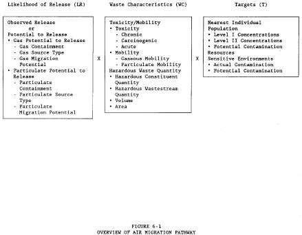
| Factor categories and factors | Maximum value | Value assigned |
| Likelihood of Release | ||
| 1. Observed Release | 550 | __ |
| 2. Potential to Release: | ||
| 2a. Gas Potential to Release | 500 | __ |
| 2b. Particulate Potential to Release | 500 | __ |
| 2c. Potential to Release (higher of lines 2a and 2b) | 500 | __ |
| 3. Likelihood of Release (higher of lines 1 and 2c) | 550 | __ |
| Waste Characteristics | ||
| 4. Toxicity/Mobility | (a) | __ |
| 5. Hazardous Waste Quantity | (a) | __ |
| 6. Waste Characteristics | 100 | __ |
| Targets | ||
| 7. Nearest Individual | 50 | __ |
| 8. Population: | ||
| 8a. Level I Concentrations | (b) | __ |
| 8b. Level II Concentrations | (b) | __ |
| 8c. Potential Contamination | (b) | __ |
| 8d. Population (lines 8a+8b+8c) | (b) | __ |
| 9. Resources | 5 | __ |
| 10. Sensitive Environments | ||
| 10a. Actual Contamination | (c) | __ |
| 10b. Potential Contamination | (c) | __ |
| 10c. Sensitive Environments (lines 10a+10b) | (c) | __ |
| 11. Targets (lines 7+8d+9+10c) | (b) | __ |
| Air Migration Pathway Score | ||
| 12. Pathway Score (S a) [(lines 3×6×11)/82,500] d | 100 | __ |
a Maximum value applies to waste characteristics category.
b Maximum value not applicable.
c No specific maximum value applies to factor. However, pathway score based solely on sensitive environments is limited to maximum of 60.
d Do not round to nearest integer.
6.1 Likelihood of Release. Evaluate the likelihood of release factor category in terms of an observed release factor or a potential to release factor.
6.1.1 Observed release. Establish an observed release to the atmosphere by demonstrating that the site has released a hazardous substance to the atmosphere. Base this demonstration on either:
- Direct observation—a material (for example, particulate matter) that contains one or more hazardous substances has been seen entering the atmosphere directly. When evidence supports the inference of a release of a material that contains one or more hazardous substances by the site to the atmosphere, demonstrated adverse effects accumulated with that release may be used to establish an observed release.
- Chemical analysis—an analysis of air samples indicates that the concentration of ambient hazardous substance(s) has increased significantly above the background concentration for the site (see section 2.3). Some portion of the significant increase must be attributable to the site to establish the observed release.
If an observed release can be established, assign an observed release factor value of 550, enter this value in Table 6-1, and proceed to section 6.1.3. If an observed release cannot be established, assign an observed release factor value of 0, enter this value in Table 6-1, and proceed to section 6.1.2.
6.1.2 Potential to release. Evaluate potential to release only if an observed release cannot be established. Determine the potential to release factor value for the site by separately evaluating the gas potential to release and the particulate potential to release for each source at the site. Select the highest potential to release value (either gas or particulate) calculated for the sources evaluated and assign that value as the site potential to release factor value as specified below.
6.1.2.1 Gas potential to release. Evaluate gas potential to release for those sources that contain gaseous hazardous substances-that is, those hazardous substances with a vapor pressure greater than or equal to 10 -9 torr.
Evaluate gas potential to release for each source based on three factors: gas containment, gas source type, and gas migration potential. Calculate the gas potential to release value as illustrated in Table 6-2. Combine sources with similar characteristics into a single source in evaluating the gas potential to release factors.
| Source | Source type a | Gas containment factor value b | Gas source type factor value c | Gas migration potential factor value d | Sum | Gas source value |
| A | B | C | (B+C) | A(B+C) | ||
| 1. | ||||||
| 2. | ||||||
| 3. | ||||||
| 4. | ||||||
| 5. | ||||||
| 6. | ||||||
| 7. | ||||||
| 8. | ||||||
| Gas Potential to Release Factor (Select the Highest Gas Source Value) | ||||||
a Enter a Source Type listed in table 6–4.
b Enter Gas Containment Factor Value from section 6.1.2.1.1.
c Enter Gas Source Type Factor Value from section 6.1.2.1.2.
d Enter Gas Migration Potential Factor Value from section 6.1.2.1.3.
6.1.2.1.1 Gas containment. Assign each source a value from Table 6-3 for gas containment. Use the lowest value from Table 6-3 that applies to the source, except: assign a value of 10 if there is evidence of biogas release or if there is an active fire within the source.
| Gas containment description | Assigned value |
| All situations except those specifically listed below | 10 |
| Evidence of biogas release | 10 a |
| Active fire within source | 10 a |
| Gas collection/treatment system functioning, regularly inspected, maintained, and completely covering source | 0 |
| Source substantially surrounded by engineering windbreak and no other containment specifically described in this table applies | 7 |
| Source covered with essentially impermeable, regularly inspected, maintained cover | 0 |
| Uncontaminated soil cover >3 feet: | |
| • Source substantially vegetated with little exposed soil | 0 |
| • Source lightly vegetated with much exposed soil | 3 |
| • Source substantially devoid of vegetation | 7 |
| Uncontaminated soil cover ≥1 foot and ≥3 feet: | |
| • Source heavily vegetated with essentially no exposed soil | |
| -Cover soil type resistant to gas migration b | 3 |
| -Cover soil type not resistant to gas migration b or unknown | 7 |
| • Source substantially vegetated with little exposed soil and cover soil type resistant to gas migration b | 7 |
| • Other | 10 |
| Uncontaminated soil cover <1 foot: | |
| • Source heavily vegetated with essentially no exposed soil and cover soil type resistant to gas migration b | 7 |
| • Other | 10 |
| Totally or partially enclosed within structurally intact building and no other containment specifically described in this table applies | 7 |
| Source consists solely of intact, sealed containers: | |
| • Totally protected from weather by regularly inspected, maintained cover | 0 |
| • Other | 3 |
a This value must be used if applicable.
b Consider moist fine-grained and saturated coarse-grained soils resistant to gas migration. Consider all other soils nonresistant.
6.1.2.1.2 Gas source type. Assign a value for gas source type to each source as follows:
- Determine if the source meets the minimum size requirement based on the source hazardous waste quantity value (see section 2.4.2.1.5). If the source receives a source hazardous waste quantity value of 0.5 or more, consider the source to meet the minimum size requirement.
- If the source meets the minimum size requirement, assign it a value from Table 6-4 for gas source type.
- If the source does not meet the minimum size requirement, assign it a value of 0 for gas source type.
If no source at the site meets the minimum size requirement, assign each source at the site a value from Table 6-4 for gas source type.
| Source type | Assigned value | |
| Gas | Particulate | |
| Active fire area | 14 | 30 |
| Burn pit | 19 | 22 |
| Containers or tanks (buried/below-ground): | ||
| • Evidence of biogas release | 33 | 22 |
| • No evidence of biogas release | 11 | 22 |
| Containers or tanks, not elsewhere specified | 28 | 14 |
| Contaminated soil (excluding land treatment) | 19 | 22 |
| Landfarm/land treatment | 28 | 22 |
| Landfill: | ||
| • Evidence of biogas release | 33 | 22 |
| • No evidence of biogas release | 11 | 22 |
| Pile: | ||
| • Tailings pile | 6 | 28 |
| • Scrap metal or junk pile | 6 | 17 |
| • Trash pile | 6 | 6 |
| • Chemical waste pile | 11 | 28 |
| • Other waste piles | 17 | 28 |
| Surface impoundments (buried/backfilled): | ||
| • Evidence of biogas release | 33 | 22 |
| • No evidence of biogas release | 11 | 22 |
| Surface impoundment (not buried/backfilled): | ||
| • Dry | 19 | 22 |
| • Other | 28 | 0 |
| Other types of sources, not elsewhere specified | 0 | 0 |
6.1.2.1.3 Gas migration potential. Evaluate this factor for each source as follows:
-
Assign a value for gas migration potential to each of the gaseous hazardous substances associated with the source (see section 2.2.2) as follows:
- Assign values from Table 6-5 for vapor pressure and Henry's constant to each hazardous substance. If Henry's constant cannot be determined for a hazardous substance, assign that hazardous substance a value of 2 for the Henry's constant component.
- Sum the two values assigned to the hazardous substance.
- Based on this sum, assign the hazardous substance a value from Table 6-6 for gas migration potential.
-
Assign a value for gas migration potential to each source as follows:
-
Select three hazardous substances associated with the source:
- If more than three gaseous hazardous substances can be associated with the source, select three that have the highest gas migration potential values.
- If fewer than three gaseous hazardous substances can be associated with a source, select all of them.
- Average the gas migration potential values assigned to the selected hazardous substances.
- Based on this average value, assign the source a gas migration potential value from Table 6-7.
-
Select three hazardous substances associated with the source:
| Vapor pressure (Torr) | Assigned value |
| Greater than 10 | 3 |
| Greater than 10 −3 to 10 | 2 |
| 10 −5 to 10 −3 | 1 |
| Less than 10 −5 | 0 |
| Henry's constant (atm-m 3 /mol) | Assigned value |
| Greater than 10 −3 | 3 |
| Greater than 10 −5 to 10 −3 | 2 |
| 10 −7 to 10 −5 | 1 |
| Less than 10 −7 | 0 |
| Sum of values for vapor pressure and Henry's constant | Assigned value |
| 0 | 0 |
| 1 or 2 | 6 |
| 3 or 4 | 11 |
| 5 or 6 | 17 |
| Average of gas migration potential values for three hazardous substances a | Assigned value |
| 0 to < 3 | 0 |
| 3 to < 8 | 6 |
| 8 to < 14 | 11 |
| 14 to 17 | 17 |
a If fewer than three hazardous substances can be associated with the source, compute the average based only on those hazardous substances that can be associated.
6.1.2.1.4 Calculation of gas potential to release value. Determine the gas potential to release value for each source as illustrated in Table 6-2. For each source, sum the gas source type factor value and gas migration potential factor value and multiply this sum by the gas containment factor value. Select the highest product calculated for the sources evaluated and assign it as the gas potential to release value for the site. Enter this value in Table 6-1.
6.1.2.2 Particulate potential to release. Evaluate particulate potential to release for those sources that contain particulate hazardous substances- that is, those hazardous substances with a vapor pressure less than or equal to 10 -1 torr.
Evaluate particulate potential to release for each source based on three factors: particulate containment, particulate source type, and particulate migration potential. Calculate the particulate potential to release value as illustrated in Table 6-8. Combine sources with similar characteristics into a single source in evaluating the particulate potential to release factors.
6.1.2.2.1 Particulate containment. Assign each source a value from Table 6-9 for particulate containment. Use the lowest value from Table 6-9 that applies to the source.
6.1.2.2.2 Particulate source type. Assign a value for particulate source type to each source in the same manner as specified for gas sources in section 6.1.2.1.2.
6.1.2.2.3 Particulate migration potential. Based on the site location, assign a value from Figure 6-2 for particulate migration potential. Assign this same value to each source at the site.
| Source | Source type a | Particulate containment factor value b | Particulate type factor value c | Particulate migration potential factor value d | Sum | Particulate source value |
| A | B | C | (B+C) | A (B+C) | ||
| 1. | ||||||
| 2. | ||||||
| 3. | ||||||
| 4. | ||||||
| 5. | ||||||
| 6. | ||||||
| 7. | ||||||
| 8. | ||||||
| Particulate Potential to Release Factor Value (Select Highest Particulate Source Value) | ||||||
a Enter a Source Type listed in table 6–4.
b Enter Particulate Containment Factor Value from section 6.1.2.2.1.
c Enter Particulate Source Type Factor Value from section 6.1.2.2.2.
d Enter Particulate Migration Potential Factor Value from section 6.1.2.2.3.
| Particulate containment description | Assigned value |
| All situations except those specifically listed below | 10 |
| Source contains only particulate hazardous substances totally covered by liquids | 0 |
| Source substantially surrounded by engineered windbreak and no other containment specifically described in this table applies | 7 |
| Source covered with essentially impermeable, regularly inspected, maintained cover | 0 |
| Uncontaminated soil cover > 3 feet: | |
| • Source substantially vegetated with little or no exposed soil | 0 |
| • Source lightly vegetated with much exposed soil | 3 |
| • Source substantially devoid of vegetation | 7 |
| Uncontaminated soil cover ≥ 1 foot and ≤ 3 feet: | |
| • Source heavily vegetated with essentially no exposed soil: | |
| -Cover soil type resistant to gas migration a | 3 |
| -Cover soil type not resistant to gas migration a or unknown | 7 |
| • Source substantially vegetated with little exposed soil and cover soil type resistant to gas migration a | 7 |
| • Other | 10 |
| Uncontaminated soil cover < 1 foot: | |
| • Source heavily vegetated with essentially no exposed soil and cover soil type resistant to gas migration a | 7 |
| • Other | 10 |
| Totally or partially enclosed within structurally intact building and no other containment specifically described in this table applies | 7 |
| Source consists solely of containers: | |
| • All containers contain only liquids | 0 |
| • All containers intact, sealed, and totally protected from weather by regularly inspected, maintained cover | 0 |
| • All containers intact and sealed | 3 |
| • Other | 10 |
a Consider moist fine-grained and saturated coarse-grained soils resistant to gas migration. Consider all other soils nonresistant.
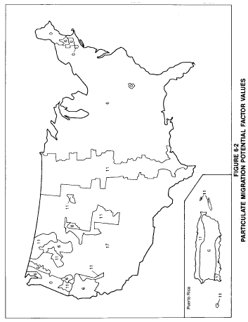
Figure 6-2—Particulate Migration Potential Factor Values—Concluded
| Location | Particulate migration potential assigned value |
| Hawaiian Islands | |
| Hilo, Hawaii | 0 |
| Honolulu, Oahu | 17 |
| Kahului, Maui | 17 |
| Lanai | 17 |
| Lihue, Kauai | 11 |
| Molokai | 17 |
| Pacific Islands | |
| Guam | 6 |
| Johnston Island | 17 |
| Koror Island | 0 |
| Kwajalein Island | 6 |
| Mujuro, Marshall Islands | 0 |
| Pago Pago, American Samoa | 0 |
| Ponape Island | 0 |
| Truk, Caroline Islands | 0 |
| Wake Island | 17 |
| Yap Island | 0 |
| Alaska | |
| Anchorage | 17 |
| Annette | 0 |
| Barrow | 17 |
| Barter Island | 17 |
| Bethel | 17 |
| Bettles | 17 |
| Big Delta | 17 |
| Cold Bay | 6 |
| Fairbanks | 17 |
| Gulkana | 17 |
| Homer | 11 |
| Juneau | 0 |
| King Salmon | 11 |
| Kodiak | 0 |
| Kutzebue | 17 |
| McGrath | 17 |
| Nome | 11 |
| St. Paul Island | 11 |
| Talkeetna | 6 |
| Unalakleet | 17 |
| Valdez | 0 |
| Yakutat | 0 |
| American Virgin Islands | |
| St. Croix | 17 |
| St. John | 11 |
| St. Thomas | 11 |
| Puerto Rico | |
| Arecibo | 6 |
| Coloso | 6 |
| Fajardo | 11 |
| Humacao | 6 |
| Isabela Station | 11 |
| Ponce | 17 |
| San Juan | 11 |
For site locations not on Figure 6-2, and for site locations near the boundary points on Figure 6-2, assign a value as follows. First, calculate a Thornthwaite P-E index using the following equation:
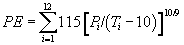
where:
PE = Thornthwaite P-E index.
P i = Mean monthly precipitation for month i, in inches.
T i = Mean monthly temperature for month i, in degrees Fahrenheit; for any month having a mean monthly temperature less than 28.4°F, use 28.4°F.
Based on the calculated Thornthwaite P-E index, assign a source particulate migration potential value to the site from Table 6-10. Assign this same value to each source at the site.
| Thornthwaite P-E Index | Assigned value |
| Greater than 150 | 0 |
| 85 to 150 | 6 |
| 50 to less than 85 | 11 |
| Less than 50 | 17 |
6.1.2.2.4 Calculation of particulate potential to release value. Determine the particulate potential to release value for each source as illustrated in Table 6-8. For each source, sum its particulate source type factor value and particulate migration potential factor value and multiply this sum by its particulate containment factor value. Select the highest product calculated for the sources evaluated and assign it as the particulate potential to release value for the site. Enter the value in Table 6-1.
6.1.2.3 Calculation of potential to release factor value for the site. Select the higher of the gas potential to release value assigned in section 6.1.2.1.4 and the particulate potential to release value assigned in section 6.1.2.2.4. Assign the value selected as the site potential to release factor value. Enter this value in Table 6-1.
6.1.3 Calculation of likelihood of release factor category value. If an observed release is established, assign the observed release factor value of 550 as the likelihood of release factor category value. Otherwise, assign the site potential to release factor value as the likelihood of release factor category value. Enter the value in Table 6-1.
6.2 Waste characteristics. Evaluate the waste characteristics factor category based on two factors: toxicity/mobility and hazardous waste quantity. Evaluate only those hazardous substances available to migrate from the sources at the site to the atmosphere. Such hazardous substances include:
- Hazardous substances that meet the criteria for an observed release to the atmosphere.
- All gaseous hazardous substances associated with a source that has a gas containment factor value greater than 0 (see section 2.2.2, 2.2.3, and 6.1.2.1.1).
- All particulate hazardous substances associated with a source that has a particulate containment factor value greater than 0 (see section 2.2.2, 2.2.3, and 6.1.2.2.1).
6.2.1 Toxicity/mobility. For each hazardous substance, assign a toxicity factor value, a mobility factor value, and a combined toxicity/mobility factor value as specified below. Select the toxicity/mobility factor value for the air migration pathway as specified in section 6.2.1.3.
6.2.1.1 Toxicity. Assign a toxicity factor value to each hazardous substance as specified in section 2.4.1.1.
6.2.1.2 Mobility. Assign a mobility factor value to each hazardous substance as follows:
-
Gaseous hazardous substance.
- Assign a mobility factor value of 1 to each gaseous hazardous substance that meets the criteria for an observed release to the atmosphere.
- Assign a mobility factor value from Table 6-11, based on vapor pressure, to each gaseous hazardous substance that does not meet the criteria for an observed release.
-
Particulate hazardous substance.
- Assign a mobility factor value of 0.02 to each particulate hazardous substance that meets the criteria for an observed release to the atmosphere.
- Assign a mobility factor value from Figure 6-3, based on the site's location, to each particulate hazardous substance that does not meet the criteria for an observed release. (Assign all such particulate hazardous substances this same value.)
-
For site locations not on Figure 6-3 and for site locations near the boundary points on Figure 6-3, assign a mobility factor value to each particulate hazardous substance that does not meet the criteria for an observed release as follows:
- Calculate a value M:
M=0.0182 (U 3 /[PE] 2)
where:
U = Mean average annual wind speed (meters per second).
PE = Thornthwaite P-E index from section 6.1.2.2.3.
- Calculate a value M:
-Based on the value M, assign a mobility factor value from table 6-12 to each particulate hazardous substance.
-
Gaseous and particulate hazardous substances.
- For a hazardous substance potentially present in both gaseous and particulate forms, select the higher of the factor values for gas mobility and particulate mobility for that substance and assign that value as the mobility factor value for the hazardous substance.
6.2.1.3 Calculation of toxicity/mobility factor value. Assign each hazardous substance a toxicity/mobility factor value from Table 6-13, based on the values assigned to the hazardous substance for the toxicity and mobility factors. Use the hazardous substance with the highest toxicity/mobility factor value to assign the value to the toxicity/mobility factor for the air migration pathway. Enter this value in Table 6-1.
| Vapor pressure (Torr) | Assigned value a |
| Greater than 10 −1 | 1.0 |
| Greater than 10 −3 to 10 −1 | 0.2 |
| Greater than 10 −5 to 10 −3 | 0.02 |
| Greater than 10 −7 to 10 −5 | 0.002 |
| Less than or equal to 10 −7 | 0.0002 |
a Do not round to nearest integer.
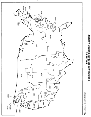
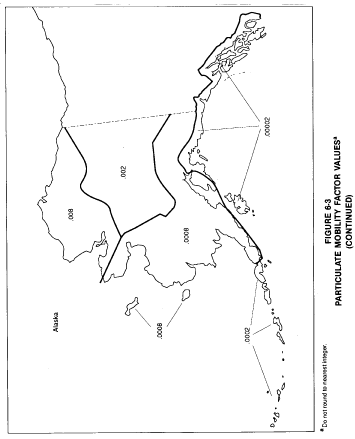
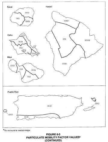
| Location | Particulated mobility assigned value |
| Pacific Islands | |
| Guam | 0.0002 |
| Johnston Island | 0.002 |
| Koror Island | 0.00008 |
| Kwajalein Island | 0.0002 |
| Mujuro, Marshall Islands | 0.00008 |
| Pago Pago, American Samoa | 0.00008 |
| Ponape Island | 0.00002 |
| Truk, Caroline Islands | 0.00008 |
| Wake Island | 0.002 |
| Yap Island | 0.00008 |
| American Virgin Islands | |
| St. Croix | 0.0008 |
| St. John | 0.0002 |
| St. Thomas | 0.0002 |
| M | Assigned value a |
| Greater than 1.4×10 −2 | 0.02 |
| Greater than 4.4×10 −3 to 1.4×10 −2 | 0.008 |
| Greater than 1.4×10 −3 to 4.4×10 −3 | 0.002 |
| Greater than 4.4×10 −4 to 1.4×10 −3 | 0.0008 |
| Greater than 1.4×10 −4 to 4.4×10 −4 | 0.0002 |
| Greater than 4.4×10 −5 to 1.4×10 −4 | 0.00008 |
| Less than or equal to 4.4×10 −5 | 0.00002 |
a Do not round to nearest integer.
| Mobility factor value | Toxicity factor value | |||||
| 10,000 | 1,000 | 100 | 10 | 1 | 0 | |
| 1.0 | 10,000 | 1,000 | 100 | 10 | 1 | 0 |
| 0.2 | 2,000 | 200 | 20 | 2 | 0.2 | 0 |
| 0.02 | 200 | 20 | 2 | 0.2 | 0.02 | 0 |
| 0.008 | 80 | 8 | 0.8 | 0.08 | 0.008 | 0 |
| 0.002 | 20 | 2 | 0.2 | 0.02 | 0.002 | 0 |
| 0.0008 | 8 | 0.8 | 0.08 | 0.008 | 0.0008 | 0 |
| 0.0002 | 2 | 0.2 | 0.02 | 0.002 | 0.0002 | 0 |
| 0.00008 | 0.8 | 0.08 | 0.008 | 0.0008 | 0.00008 | 0 |
| 0.00002 | 0.2 | 0.02 | 0.002 | 0.0002 | 0.00002 | 0 |
a Do not round to nearest integer.
6.2.2 Hazardous waste quantity. Assign a hazardous waste quantity factor value for the air migration pathway as specified in section 2.4.2. Enter this value in Table 6-1.
6.2.3 Calculation of waste characteristics factor category value. Multiply the toxicity/mobility factor value and the hazardous waste quantity factor value, subject to a maximum product of 1 x 10 8. Based on this product, assign a value from Table 2-7 (section 2.4.3.1) to the waste characteristics factor category. Enter this value in Table 6-1.
6.3 Targets.
Evaluate the targets factor category based on four factors: nearest individual, population, resources, and sensitive environments. Include only those targets (for example, individuals, sensitive environments) located within the 4-mile target distance limit, except: if an observed release is established beyond the 4-mile target distance limit, include those additional targets that are specified below in this section and in section 6.3.4.
Evaluate the nearest individual and population factors based on whether the target populations are subject to Level I concentrations, Level II concentrations, or potential contamination. Determine which applies to a target population as follows.
If no samples meet the criteria for an observed release to air and if there is no observed release by direct observation, consider the entire population within the 4-mile target distance limit to be subject to potential contamination.
If one or more samples meet the criteria for an observed release to air or if there is an observed release by direct observation, evaluate the population as follows:
- Determine the most distant sample location that meets the criteria for Level I concentrations as specified in sections 2.5.1 and 2.5.2 and the most distant location (that is, sample location or direct observation location) that meets the criteria for Level II concentrations. Use the health-based benchmarks from Table 6-14 in determining the level of contamination for sample locations. If the most distant Level II location is closer to a source than the most distant Level I sample location, do not consider the Level II location.
- Determine the single most distant location (sample location or direct observation location) that meets the criteria for Level I or Level II concentrations.
-
If this single most distant location is within the 4-mile target distance limit, identify the distance categories from Table 6-15 in which the selected Level I concentrations sample and Level II concentrations sample (or direct observation location) are located:
- Consider the target population anywhere within this furthest Level I distance category, or anywhere within a distance category closer to a source at the site, as subject to Level I concentrations.
- Consider the target population located beyond any Level I distance categories, up to and including the population anywhere within the furthest Level II distance category, as subject to Level II concentrations.
- Consider the remainder of the target population within the 4-mile target distance limit as subject to potential contamination.
-
If the single most distant location is beyond the 4-mile target distance limit, identify the distance at which the selected Level I concentrations sample and Level II concentrations sample (or direct observation location) are located:
- If the Level I sample location is within the 4-mile target distance limit, identify the target population subject to Level I concentrations as specified above.
- If the Level I sample location is beyond the 4-mile target distance limit, consider the target population located anywhere within a distance from the sources at the site equal to the distance to this sample location to be subject to Level I concentrations and include them in the evaluation.
- Consider the target population located beyond the Level I target population, but located anywhere within a distance from the sources at the site equal to the distance to the selected Level II location, to be subject to Level II concentrations and include them in the evaluation.
- Do not include any target population as subject to potential contamination.
| • Concentration corresponding to National Ambient Air Quality Standard (NAAQS). |
| • Concentration corresponding to National Emission Standards for Hazardous Air Pollutants (NESHAPs). |
| • Screening concentration for cancer corresponding to that concentration that corresponds to the 10 −6 individual cancer risk for inhalation exposures. |
| • Screening concentration for noncancer toxicological responses corresponding to the Reference Concentration (RfC) for inhalation exposures. |
| Distance category (miles) | Assigned distance weight a |
| 0 | 1.0 |
| Greater than 0 to 1/4 | 0.25 |
| Greater than 1/4 to 1/2 | 0.054 |
| Greater than 1/2 to 1 | 0.016 |
| Greater than 1 to 2 | 0.0051 |
| Greater than 2 to 3 | 0.0023 |
| Greater than 3 to 4 | 0.0014 |
| Greater than 4 | 0 |
a Do not round to nearest integer.
6.3.1 Nearest individual. Assign the nearest individual factor a value as follows:
- If one or more residences or regularly occupied buildings or areas is subject to Level I concentrations as specified in section 6.3, assign a value of 50.
- If not, but if one or more a residences or regularly occupied buildings or areas is subject to Level II concentrations, assign a value of 45.
- If none of the residences and regularly occupied buildings and areas is subject to Level I or Level II concentrations, assign a value to this factor based on the shortest distance to any residence or regularly occupied building or area, as measured from any source at the site with an air migration containment factor value greater than 0. Based on this shortest distance, assign a value from Table 6-16 to the nearest individual factor.
Enter the value assigned in Table 6-1.
| Distance to nearest individual (miles) | Assigned value |
| Level I concentrations a | 50 |
| Level II concentrations a | 45 |
| 0 to 1/8 | 20 |
| Greater than 1/8 to 1/4 | 7 |
| Greater than 1/4 to 1/2 | 2 |
| Greater than 1/2 to 1 | 1 |
| Greater than 1 | 0 |
a Distance does not apply.
6.3.2 Population. In evaluating the population factor, count residents, students, and workers regularly present within the target distance limit. Do not count transient populations such as customers and travelers passing through the area.
In estimating residential population, when the estimate is based on the number of residences, multiply each residence by the average number of persons per residence for the county in which the residence is located.
6.3.2.1 Level of contamination. Evaluate the population factor based on three factors: Level I concentrations, Level II concentrations, and potential contamination.
Evaluate the population subject to Level I concentrations (see section 6.3) as specified in section 6.3.2.2, the population subject to Level II concentrations as specified in section 6.3.2.3, and the population subject to potential contamination as specified in section 6.3.2.4.
For the potential contamination factor, use population ranges in evaluating the factor as specified in section 6.3.2.4. For the Level I and Level II concentrations factors, use the population estimate, not population ranges, in evaluating both factors.
6.3.2.2 Level I concentrations. Sum the number of people subject to Level I concentrations. Multiply this sum by 10. Assign the product as the value for this factor. Enter this value in Table 6-1.
6.3.2.3 Level II concentrations. Sum the number of people subject to Level II concentrations. Do not include those people already counted under the Level I concentrations factor. Assign this sum as the value for this factor. Enter this value in Table 6-1.
6.3.2.4 Potential contamination. Determine the number of people within each distance category of the target distance limit (see Table 6-15) who are subject to potential contamination. Do not include those people already counted under the Level I and Level II concentrations factors.
Based on the number of people present within a distance category, assign a distance-weighted population value for that distance category from Table 6- 17. (Note that the distance-weighted population values in Table 6-17 incorporate the distance weights from Table 6-15. Do not multiply the values from Table 6-17 by these distance weights.)
Calculate the potential contamination factor value (PI) as follows:

where:
W i = Distance-weighted population from Table 6-17 for distance category i.
n = Number of distance categories.
If PI is less than 1, do not round it to the nearest integer; if PI is 1 or more, round to the nearest integer. Enter this value in Table 6-1.
6.3.2.5 Calculation of population factor value. Sum the factor values for Level I concentrations, Level II concentrations, and potential contamination. Do not round this sum to the nearest integer. Assign this sum as the population factor value. Enter this value in Table 6-1.
| Distance category (miles) | Number of people within the distance category | ||||||||||||
| 0 | 1 to 10 | 11 to 30 | 31 to 100 | 101 to 300 | 301 to 1,000 | 1,001 to 3,000 | 3,001 to 10,000 | 10,001 to 30,000 | 30,001 to 100,000 | 100,001 to 300,000 | 300,001 to 1,000,000 | 1,000,001 to 3,000,000 | |
| On a source | 0 | 4 | 17 | 53 | 164 | 522 | 1,633 | 5,214 | 16,325 | 52,137 | 163,246 | 521,360 | 1,632,455 |
| Greater than 0 to 1/4 | 0 | 1 | 4 | 13 | 41 | 131 | 408 | 1,304 | 4,081 | 13,034 | 40,812 | 130,340 | 408,114 |
| Greater than 1/4 to 1/2 | 0 | 0.2 | 0.9 | 3 | 9 | 28 | 88 | 282 | 882 | 2,815 | 8,815 | 28,153 | 88,153 |
| Greater than 1/2 to 1 | 0 | 0.06 | 0.3 | 0.9 | 3 | 8 | 26 | 83 | 261 | 834 | 2,612 | 8,342 | 26,119 |
| Greater than 1 to 2 | 0 | 0.02 | 0.09 | 0.3 | 0.8 | 3 | 8 | 27 | 83 | 266 | 833 | 2,659 | 8,326 |
| Greater than 2 to 3 | 0 | 0.009 | 0.04 | 0.1 | 0.4 | 1 | 4 | 12 | 38 | 120 | 375 | 1,199 | 3,755 |
| Greater than 3 to 4 | 0 | 0.005 | 0.02 | 0.07 | 0.2 | 0.7 | 2 | 7 | 23 | 73 | 229 | 730 | 2,285 |
a Round the number of people present within a distance category to nearest integer. Do not round the assigned distance-weighted population value to nearest integer.
6.3.3 Resources. Evaluate the resources factor as follows:
-
Assign a value of 5 if one or more of the following resources are present within one-half mile of a source at the site having an air migration containment factor value greater than 0:
- Commercial agriculture.
- Commercial silviculture.
- Major or designated recreation area.
- Assign a value of 0 if none of these resources is present.
Enter the value assigned in Table 6-1.
6.3.4 Sensitive environments. Evaluate sensitive environments based on two factors: actual contamination and potential contamination. Determine which factor applies as follows.
If no samples meet the criteria for an observed release to air and if there is no observed release by direct observation, consider all sensitive environments located, partially or wholly, within the target distance limit to be subject to potential contamination.
If one or more samples meet the criteria for an observed release to air or if there is an observed release by direct observation, determine the most distant location (that is, sample location or direct observation location) that meets the criteria for an observed release:
-
If the most distant location meeting the criteria for an observed release is within the 4-mile target distance limit, identify the distance category from Table 6-15 in which it is located:
- Consider sensitive environments located, partially or wholly, anywhere within this distance category or anywhere within a distance category closer to a source at the site as subject to actual contamination.
- Consider all other sensitive environments located, partially or wholly, within the target distance limit as subject to potential contamination.
-
If the most distant location meeting the criteria for an observed release is beyond the 4-mile target distance limit, identify the distance at which it is located:
- Consider sensitive environments located, partially or wholly, anywhere within a distance from the sources at the site equal to the distance to this location to be subject to actual contamination and include all such sensitive environments in the evaluation.
- Do not include any sensitive environments as subject to potential contamination.
6.3.4.1 Actual contamination. Determine those sensitive environments subject to actual contamination (i.e., those located partially or wholly within a distance category subject to actual contamination). Assign value(s) from Table 4-23 (section 4.1.4.3.1.1) to each sensitive environment subject to actual contamination.
For those sensitive environments that are wetlands, assign an additional value from Table 6-18. In assigning a value from Table 6-18, include only those portions of wetlands located within distance categories subject to actual contamination. If a wetland is located partially in a distance category subject to actual contamination and partially in one subject to potential contamination, then solely for purposes of Table 6-18, count the portion in the distance category subject to potential contamination under the potential contamination factor in section 6.3.4.2. Determine the total acreage of wetlands within those distance categories subject to actual contamination and assign a value from Table 6-18 based on this total acreage.
Calculate the actual contamination factor value (EA) as follows:
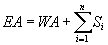
where:
WA = Value assigned from Table 6-18 for wetlands in distance categories subject to actual contamination.
S i = Value(s) assigned from Table 4-23 to sensitive environment i.
n = Number of sensitive environments subject to actual contamination.
Enter the value assigned in Table 6-1.
| Wetland area (acres) | Assigned value |
| Less than 1 | 0 |
| 1 to 50 | 25 |
| Greater than 50 to 100 | 75 |
| Greater than 100 to 150 | 125 |
| Greater than 150 to 200 | 175 |
| Greater than 200 to 300 | 250 |
| Greater than 300 to 400 | 350 |
| Greater than 400 to 500 | 450 |
| Greater than 500 | 500 |
a Wetlands as defined in 40 CFR section 230.3.
6.3.4.2 Potential contamination. Determine those sensitive environments located, partially or wholly, within the target distance limit that are subject to potential contamination. Assign value(s) from Table 4-23 to each sensitive environment subject to potential contamination. Do not include those sensitive environments already counted for Table 4-23 under the actual contamination factor.
For each distance category subject to potential contamination, sum the value(s) assigned from Table 4-23 to the sensitive environments in that distance category. If a sensitive environment is located in more than one distance category, assign the sensitive environment only to that distance category having the highest distance weighting value from Table 6-15.
For those sensitive environments that are wetlands, assign an additional value from Table 6-18. In assigning a value from Table 6-18, include only those portions of wetlands located within distance categories subject to potential contamination, as specified in section 6.3.4.1. Treat the wetlands in each separate distance category as separate sensitive environments solely for purposes of applying Table 6-18. Determine the total acreage of wetlands within each of these distance categories and assign a separate value from Table 6-18 for each distance category.
Calculate the potential contamination factor value (EP) as follows:
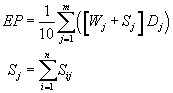
S ij = Value(s) assigned from Table 4-23 to sensitive environment in distance category j.
n = Number of sensitive environments subject to potential contamination.
W j = Value assigned from Table 6-18 for wetland area in distance category j.
D j = Distance weight from Table 6-15 for distance category j.
m = Number of distance categories subject to potential contamination.
If EP is less than 1, do not round it to the nearest integer; if EP is 1 or more, round to the nearest integer. Enter the value assigned in Table 6-1.
6.3.4.3 Calculation of sensitive environments factor value. Sum the factor values for actual contamination and potential contamination. Do not round this sum, designated as EB, to the nearest integer.
Because the pathway score based solely on sensitive environments is limited to a maximum of 60, use the value EB to determine the value for the sensitive environments factor as follows:
-
Multiply the values assigned to likelihood of release (LR), waste characteristics (WC), and EB. Divide the product by 82,500.
- If the result is 60 or less, assign the value EB as the sensitive environments factor value.
- If the result exceeds 60, calculate a value EC as follows:
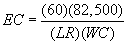
Assign the value EC as the sensitive environments factor value. Do not round this value to the nearest integer.
Enter the value assigned for the sensitive environments factor in Table 6- 1.
6.3.5 Calculation of targets factor category value. Sum the nearest individual, population, resources, and sensitive environments factor values. Do not round this sum to the nearest integer. Assign this sum as the targets factor category value. Enter this value in Table 6-1.
6.4 Calculation of air migration pathway score. Multiply the values for likelihood of release, waste characteristics, and targets, and round the product to the nearest integer. Then divide by 82,500. Assign the resulting value, subject to a maximum value of 100, as the air migration pathway score (S a). Enter this score in Table 6-1.
7.0 Sites Containing Radioactive Substances.
In general, radioactive substances are hazardous substances under CERCLA and should be considered in HRS scoring. Releases of certain radioactive substances are, however, excluded from the definition of "release" in section 101(22) of CERCLA, as amended, and should not be considered in HRS scoring.
Evaluate sites containing radioactive substances using the instructions specified in sections 2 through 6, supplemented by the instructions in this section. Those factors denoted with a "yes" in Table 7-1 are evaluated differently for sites containing radioactive substances than for sites containing only nonradioactive hazardous substances, while those denoted with a "no" are not evaluated differently and are not addressed in this section.
| Ground water pathway | Status a | Surface water pathway | Status a | Soil exposure component of SESSI pathway | Status a | Subsurface intrusion component of SESSI pathway | Status a | Air pathway | Status a |
|---|---|---|---|---|---|---|---|---|---|
| Likelihood of Release | Likelihood of Release | Likelihood of Exposure | Likelihood of Exposure | Likelihood of Release | |||||
| Observed Release | Yes | Observed Release | Yes | Observed Contamination | Yes | Observed Exposure | Yes | Observed Release | Yes. |
| Potential to Release | No | Potential to Release | No | Attractiveness/Accessibility to Nearby Residents | No | Potential for Exposure | Yes | Gas Potential to Release | No. |
| Containment | No | Overland Flow Containment | No | Area of Contamination | No | Structure Containment | No | Gas Containment | No. |
| Net Precipitation | No | Runoff | No | Depth to Contamination | Yes | Gas Source Type | No. | ||
| Depth to Aquifer | No | Distance to Surface water | No | Vertical migration | No | Gas Migration Potential | No. | ||
| Travel Time | No | Flood Frequency | No | Vapor Migration Potential | No | Particulate Potential to Release | No. | ||
| Flood Containment | No | Area of Observed Exposure | No | Particulate Containment | No. | ||||
| Area of Subsurface Contamination | No | Particulate Source Type | No. | ||||||
| Particulate Migration Potential | No. | ||||||||
| Waste Characteristics | Waste Characteristics | Waste Characteristics | Waste Characteristics | Waste Characteristics | |||||
| Toxicity | Yes | Toxicity/Ecotoxicity | Yes/Yes | Toxicity | Yes | Toxicity/Degradation | Yes/Yes | Toxicity | Yes. |
| Mobility | No | Persistence/Mobility | Yes/No | Hazardous Waste Quantity | Yes | Hazardous Waste Quantity | Yes | Mobility | No. |
| Hazardous Waste Quantity | Yes | Bioaccumulation Potential | No | Hazardous Waste Quantity | Yes. | ||||
| Hazardous Waste Quantity | Yes | ||||||||
| Targets | Targets | Targets | Targets | Targets | |||||
| Nearest Well | Yes b | Nearest Intake | Yes b | Resident Individual | Yes b | Exposed Individual | Yes b | Nearest Individual | Yes. b |
| Population | Yes b | Drinking Water Population | Yes b | Resident Population | Yes b | Population | Yes b | Population | Yes. b |
| Resources | No | Resources | No | Workers | No | Resources | No | Resources | No. |
| Wellhead Protection Area | No | Sensitive Environments | Yes b | Resources | No | Sensitive Environments | No. | ||
| Human Food Chain Individual | Yes b | Terrestrial Sensitive Environments | No | ||||||
| Human Food Chain Population | Yes b | Nearby Individual Population Within 1 Mile | No No. | ||||||
| a—Factors evaluated differently are denoted by “yes”; factors not evaluated differently are denoted by “no”. b—Difference is in the determination of Level I and Level II concentrations. | |||||||||
In general, sites containing mixed radioactive and other hazardous substances involve more evaluation than sites containing only radionuclides. For sites containing mixed radioactive and other hazardous substances, HRS factors are evaluated based on considerations of both the radioactive substances and the other hazardous substances in order to derive a single set of factor values for each factor category in each of the four pathways. Thus, the HRS score for these sites reflects the combined potential hazards posed by both the radioactive and other hazardous substances.
Section 7 is organized by factor category, similar to sections 3 through 6. Pathway-specific differences in evaluation criteria are specified under each factor category, as appropriate. These differences apply largely to the soil exposure and subsurface intrusion pathway and to sites containing mixed radioactive and other hazardous substances.
7.1 Likelihood of release/likelihood of exposure. Evaluate likelihood of release for the three migration pathways and likelihood of exposure for the soil exposure and subsurface intrusion pathway as specified in sections 2 through 6, except: establish an observed release, observed contamination, and/or observed exposure as specified in section 7.1.1. When an observed release or exposure cannot be established for a migration pathway or the subsurface intrusion component of the soil exposure and subsurface intrusion pathway, evaluate potential to release as specified in section 7.1.2. When observed contamination cannot be established, do not evaluate the soil exposure component of the soil exposure and subsurface intrusion pathway.
7.1.1 Observed release/observed contamination/observed exposure. For radioactive substances, establish an observed release for each migration pathway by demonstrating that the site has released a radioactive substance to the pathway (or watershed or aquifer, as appropriate); establish observed contamination or observed exposure for the soil exposure and subsurface intrusion pathway as indicated below. Base these demonstrations on one or more of the following, as appropriate to the pathway being evaluated:
-
Direct observation:
- —For each migration pathway, a material that contains one or more radionuclides has been seen entering the atmosphere, surface water, or ground water, as appropriate, or is known to have entered ground water or surface water through direct deposition, or
- —For the surface water migration pathway, a source area containing radioactive substances has been flooded at a time that radioactive substances were present and one or more radioactive substances were in contact with the flood waters.
- —For the subsurface intrusion component of the soil exposure and subsurface intrusion pathway, a material that contains one or more radionuclides has been observed entering a regularly occupied structure via the subsurface or is known to have entered a regularly occupied structure via the subsurface. Also, when evidence supports the inference of subsurface intrusion of a material that contains one or more radionuclides by the site into a regularly occupied structure, demonstrated adverse effects associated with that release may also be used to establish observed exposure by direct observation.
-
Analysis of radionuclide concentrations in samples appropriate to the pathway (that is, ground water, soil, air, indoor air, soil gas, surface water, benthic, or sediment samples):
-
—For radionuclides that occur naturally and for radionuclides that are ubiquitous in the environment:
-
Measured concentration (in units of activity, for example, pCi per kilogram [pCi/kg], pCi per liter [pCi/L], pCi per cubic meter [pCi/m3]) of a given radionuclide in the sample are at a level that:
- Equals or exceeds a value 2 standard deviations above the mean site-specific background concentration for that radionuclide in that type of sample, or
- Exceeds the upper-limit value of the range of regional background concentration values for that specific radionuclide in that type of sample.
- Some portion of the increase must be attributable to the site to establish the observed release (or observed contamination or observed exposure), and
- For the soil exposure component of the soil exposure and subsurface intrusion pathway only, the radionuclide must also be present at the surface or covered by 2 feet or less of cover material (for example, soil) to establish observed contamination.
-
Measured concentration (in units of activity, for example, pCi per kilogram [pCi/kg], pCi per liter [pCi/L], pCi per cubic meter [pCi/m3]) of a given radionuclide in the sample are at a level that:
-
—For man-made radionuclides without ubiquitous background concentrations in the environment:
- Measured concentration (in units of activity) of a given radionuclide in a sample equals or exceeds the sample quantitation limit for that specific radionuclide in that type of media and is attributable to the site.
- However, if the radionuclide concentration equals or exceeds its sample quantitation limit, but its release can also be attributed to one or more neighboring sites, then the measured concentration of that radionuclide must also equal or exceed a value either 2 standard deviations above the mean concentration of that radionuclide contributed by those neighboring sites or 3 times its background concentration, whichever is lower.
-
If the sample quantitation limit cannot be established:
- If the sample analysis was performed under the EPA Contract Laboratory Program, use the EPA contract-required quantitation limit (CRQL) in place of the sample quantitation limit in establishing an observed release (or observed contamination or observed exposure).
- If the sample analysis is not performed under the EPA Contract Laboratory Program, use the detection limit in place of the sample quantitation limit.
- For the soil exposure component of the soil exposure and subsurface intrusion pathway only, the radionuclide must also be present at the surface or covered by 2 feet or less of cover material (for example, soil) to establish observed contamination.
-
—For radionuclides that occur naturally and for radionuclides that are ubiquitous in the environment:
-
Gamma radiation measurements (applies only to observed contamination or observed exposure in the soil exposure and subsurface intrusion pathway):
- —The gamma radiation exposure rate, as measured in microroentgens per hour (μR/hr) using a survey instrument held 1 meter above the ground surface or floor or walls of a structure (or 1 meter away from an aboveground source for the soil exposure component), equals or exceeds 2 times the site-specific background gamma radiation exposure rate.
- —Some portion of the increase must be attributable to the site to establish observed contamination or observed exposure. The gamma-emitting radionuclides do not have to be within 2 feet of the surface of the source.
For the three migration pathways and for the subsurface intrusion component of the soil exposure and subsurface intrusion pathway, if an observed release or observed exposure can be established for the pathway (or component, threat, aquifer, or watershed, as appropriate), assign the pathway (or component, threat, aquifer, or watershed) an observed release or observed exposure factor value of 550 and proceed to section 7.2. If an observed release or observed exposure cannot be established, assign an observed release or observed exposure factor value of 0 and proceed to section 7.1.2.
For the soil exposure component of the soil exposure and subsurface intrusion pathway, if observed contamination can be established, assign the likelihood of exposure factor for resident population a value of 550 if there is an area of observed contamination in one or more locations listed in section 5.1.1; evaluate the likelihood of exposure factor for nearby population as specified in section 5.1.2.1; and proceed to section 7.2. If observed contamination cannot be established, do not evaluate the soil exposure component of the soil exposure and subsurface intrusion pathway.
At sites containing mixed radioactive and other hazardous substances, evaluate observed release (or component, observed contamination or observed exposure) separately for radionuclides as described in this section and for other hazardous substances as described in sections 2 through 6.
For the three migration pathways and the subsurface intrusion component of the soil exposure and subsurface intrusion pathway, if an observed release or observed exposure can be established based on either radionuclides or other hazardous substances, or both, assign the pathway (or threat, aquifer, or watershed) an observed release or observed exposure factor value of 550 and proceed to section 7.2. If an observed release or observed exposure cannot be established based on either radionuclides or other hazardous substances, assign an observed release or observed exposure factor value of 0 and proceed to section 7.1.2.
For the soil exposure component of the soil exposure and subsurface intrusion pathway, if observed contamination can be established based on either radionuclides or other hazardous substances, or both, assign the likelihood of exposure factor for resident population a value of 550 if there is an area of observed contamination in one or more locations listed in section 5.1.1; evaluate the likelihood of exposure factor for nearby population as specified in section 5.1.2.1; and proceed to section 7.2. If observed contamination cannot be established based on either radionuclides or other hazardous substances, do not evaluate the soil exposure component of the soil exposure and subsurface intrusion pathway.
7.1.2 Potential to release/potential for exposure. For the three migration pathways and the subsurface intrusion component of the soil exposure and subsurface intrusion pathway, evaluate potential to release or potential for exposure for sites containing radionuclides in the same manner as specified for sites containing other hazardous substances. Base the evaluation on the physical and chemical properties of the radionuclides, not on their level of radioactivity. For the subsurface intrusion component of the soil exposure and subsurface intrusion pathway, if the potential for exposure is based on the presence of gamma emitting radioactive substances, assign a potential for exposure factor value of 500 only if the contamination is found within 2 feet beneath a regularly occupied structure, otherwise assign a potential for exposure factor value of 0.
For sites containing mixed radioactive and other hazardous substances, evaluate potential to release or potential for exposure considering radionuclides and other hazardous substances together. Evaluate potential to release for each migration pathway and the potential for exposure for the subsurface intrusion component of the soil exposure and subsurface intrusion pathway as specified in sections 3 through 6, as appropriate.
7.2 Waste characteristics. For radioactive substances, evaluate the human toxicity factor, the ecosystem toxicity factor, the surface water persistence factor, and the hazardous waste quantity factor as specified in the following sections. Evaluate all other waste characteristic factors as specified in sections 2 through 6.
7.2.1 Human Toxicity. For radioactive substances, evaluate the human toxicity factor as specified below, not as specified in section 2.4.1.1.
Assign human toxicity factor values to those radionuclides available to the pathway based on quantitative dose-response parameters for cancer risks as follows:
- Evaluate radionuclides only on the basis of carcinogenicity and assign all radionuclides to weight-of-evidence category A, or weight-of-evidence category “Carcinogenic to Humans”.
-
Assign a human toxicity factor value from Table 7-2 to each radionuclide based on its slope factor (also referred to as a cancer potency factor).
- —For each radionuclide, use the higher of the slope factors for inhalation and ingestion to assign the factor value.
- —If only one slope factor is available for the radionuclide use it to assign the toxicity factor value.
- —If no slope factor is available for the radionuclide, assign that radionuclide a toxicity factor value of 0 and use other radionuclides for which a slope factor is available to evaluate the pathway.
- If all radionuclides available to a particular pathway are assigned a human toxicity factor value of 0 (that is, no slope factor is available for all the radionuclides), use a default human toxicity factor value of 1,000 as the human toxicity factor value for all radionuclides available to the pathway.
At sites containing mixed radioactive and other hazardous substances, evaluate the toxicity factor separately for the radioactive and other hazardous substances and assign each a separate toxicity factor value. This applies regardless of whether the radioactive and other hazardous substances are physically separated, combined chemically, or simply mixed together. Assign toxicity factor values to the radionuclides as specified above and to the other hazardous substances as specified in section 2.4.1.1.
At sites containing mixed radioactive and other hazardous substances, if all radionuclides available to a particular pathway are assigned a human toxicity factor value of 0, use a default human toxicity factor value of 1,000 for all those radionuclides even if nonradioactive hazardous substances available to the pathway are assigned human toxicity factor values greater than 0. Similarly, if all nonradioactive hazardous substances available to the pathway are assigned a human toxicity factor value of 0, use a default human toxicity factor value of 100 for all these nonradioactive hazardous substances even if radionuclides available to the pathway are assigned human toxicity factor values greater than 0.
7.2.2 Ecosystem toxicity. For the surface water environmental threat (see sections 4.1.4 and 4.2.4). assign an ecosystem toxicity factor value to radionuclides (alone or combined chemically or mixed with other hazardous substances) using the same slope factors and procedures specified for the human toxicity factor in section 7.2.1, except: use a default of 100, not 1,000, if all radionuclides eligible to be evaluated for ecosystem toxicity receive an ecosystem toxicity factor value of 0.
| Cancer slope factor a (SF) (pCi) −1 | Assigned value |
| 3×10 −11 ≤ SF | 10,000 |
| 3×10 −12 ≤ SF<3×10 −11 | 1,000 |
| SF<3×10 −12 | 100 |
| SF not available for the radionuclide | 0 |
a Radionuclide slope factors are estimates of age-averaged, individual lifetime total excess cancer risk per picocurie of radionuclide inhaled or ingested.
At sites containing mixed radioactive and other hazardous substances, evaluate the ecosystem toxicity factor separately for the radioactive and other hazardous substances and assign each a separate ecosystem toxicity factor value. This applies regardless of whether the radioactive and other hazardous substances are physically separated, combined chemically, or simply mixed together. Assign ecosystem toxicity factor values to the radionuclides as specified above and to the other hazardous substances as specified in sections 4.1.4.2.1.1 and 4.2.4.2.1.1. If all radionuclides available to a particular pathway are assigned an ecosystem toxicity factor value of 0, use a default ecosystem toxicity factor value of 100 for all these radionuclides even if nonradioactive hazardous substances available to the pathway are assigned ecosystem toxicity factor values greater than 0. Similarly, if all nonradioactive hazardous substances available to the pathway are assigned an ecosystem toxicity factor value of 0, use a default ecosystem toxicity factor value of 100 for all these nonradioactive hazardous substances even if radionuclides available to the pathway are assigned ecosystem toxicity factor values greater than 0.
7.2.3 Persistence/Degradation. In determining the surface water persistence factor for radionuclides, evaluate this factor based solely on half-life; do not include sorption to sediments in the evaluation as is done for nonradioactive hazardous substances. Assign a persistence factor value from Table 4-10 (section 4.1.2.2.1.2) to each radionuclide based on half-life (t 1/2) calculated as follows:
Where:
r = Radioactive half-life.
V = Volatilization half-life.
If the volatilization half-life cannot be estimated for a radionuclide from available data, delete it from the equation. Select the portion of Table 4-10 to use in assigning the persistence factor value as specified in section 4.1.2.2.1.2.
At sites containing mixed radioactive and other hazardous substances, evaluate the persistence factor separately for each radionuclide and for each nonradioactive hazardous substance, even if the available data indicate that they are combined chemically. Assign a persistence factor value to each radionuclide as specified in this section and to each nonradioactive hazardous substance as specified in section 4.1.2.2.1.2. When combined chemically, assign a single persistence factor value based on the higher of the two values assigned (individually) to the radioactive and nonradioactive components.
In determining the subsurface intrusion degradation factor for radionuclides, when evaluating this factor based solely on half-life, assign a degradation factor value from section 5.2.1.2.1.2 to each radionuclide based on half-life (t 1/2) calculated as follows:
Where:
r=Radioactive half-life.
If no radioactive half-life information is available for a radionuclide and the substance is not already assigned a value of 1, unless information indicates otherwise, assign a value of 1.
At sites containing mixed radioactive and other hazardous substances, evaluate the degradation factor separately for each radionuclide and for each nonradioactive hazardous substance, even if the available data indicate that they are combined chemically. Assign a degradation factor value to each radionuclide as specified in this section and to each nonradioactive hazardous substance as specified in section 5.2.1.2.1.2. If no radioactive half-life information is available for a radionuclide and the substance is not already assigned a value of 1, unless information indicates otherwise, assign a value of 1. Similarly, if no half-life information is available for a nonradioactive substance, and the substance is not already assigned a value of 1, unless information indicates otherwise, assign a value of 1. When combined chemically, assign a single persistence or degradation factor value based on the higher of the two values assigned (individually) to the radioactive and nonradioactive components.
7.2.4 Selection of substance potentially posing greatest hazard. For the subsurface intrusion component of the soil exposure and subsurface intrusion pathway and each migration pathway (or threat, aquifer, or watershed, as appropriate), select the radioactive substance or nonradioactive hazardous substance that potentially poses the greatest hazard based on its toxicity factor value, combined with the applicable mobility, persistence, degradation and/or bioaccumulation (or ecosystem bioaccumulation) potential factor values. Combine these factor values as specified in sections 2 through 6. For the soil exposure component of the soil exposure and subsurface intrusion pathway, base the selection on the toxicity factor alone (see sections 2 and 5).
7.2.5 Hazardous waste quantity. To calculate the hazardous waste quantity factor value for sites containing radioactive substances, evaluate source hazardous waste quantity (see section 2.4.2.1) using only the following two measures in the following hierarchy (these measures are consistent with Tiers A and B for nonradioactive hazardous substances in sections 2.4.2.1.1 and 2.4.2.1.2):
- Radionuclide constituent quantity (Tier A).
- Radionuclide wastestream quantity (Tier B).
7.2.5.1 Source hazardous waste quantity for radionuclides. For each migration pathway, assign a source hazardous waste quantity value to each source having a containment factor value greater than 0 for the pathway being evaluated. For the soil exposure component of the soil exposure and subsurface intrusion pathway, assign a source hazardous waste quantity value to each area of observed contamination, as applicable to the threat being evaluated. For the subsurface intrusion component, assign a source hazardous waste quantity value to each regularly occupied structure located within areas of observed exposure or areas of subsurface contamination. Allocate hazardous substances and hazardous wastestreams to specific sources (or areas of observed contamination, areas of observed exposure or areas of subsurface contamination) as specified in sections 2.4.2 and 5.2.0.
7.2.5.1.1 Radionuclide constituent quantity (Tier A). Evaluate radionuclide constituent quantity for each source (or area of observed contamination or area of observed exposure) based on the activity content of the radionuclides allocated to the source (or area of observed contamination or area of observed exposure) as follows:
-
Estimate the net activity content (in curies) for the source (or area of observed contamination or area of observed exposure) based on:
- —Manifests, or
- —Either of the following equations, as applicable:
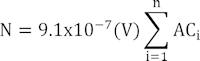
Where:
N=Estimated net activity content (in curies) for the source (or area of observed contamination or area of observed exposure).
V=Total volume of material (in cubic yards) in a source (or area of observed contamination or area of observed exposure) containing radionuclides.
AC i =Activity concentration above the respective background concentration (in pCi/g) for each radionuclide i allocated to the source (or area of observed contamination or area of observed exposure).
n=Number of radionuclides allocated to the source (or area of observed contamination or area of observed exposure) above the respective background concentrations.
or,
Where:
N=Estimated net activity content (in curies) for the source (or area of observed contamination or area of observed exposure).
V=Total volume of material (in gallons) in a source (or area of observed contamination or area of observed exposure) containing radionuclides.
AC i =Activity concentration above the respective background concentration (in pCi/1) for each radionuclide i allocated to the source (or area of observed contamination or area of observed exposure).
n=Number of radionuclides allocated to the source (or area of observed contamination or area of observed exposure) above the respective background concentrations. - —Estimate volume for the source (or volume for the area of observed contamination or area of observed exposure) based on records or measurements.
- —For the soil exposure component of the soil exposure and subsurface intrusion pathway, in estimating the volume for areas of observed contamination, do not include more than the first 2 feet of depth, except: for those types of areas of observed contamination listed in Tier C of Table 5-2 (section 5.1.1.2.2), include the entire depth, not just that within 2 feet of the surface.
- Convert from curies of radionuclides to equivalent pounds of nonradioactive hazardous substances by multiplying the activity estimate for the source (or area of observed contamination or area of observed exposure) by 1,000.
- Assign this resulting product as the radionuclide constituent quantity value for the source (or area of observed contamination or area of observed exposure).
If the radionuclide constituent quantity for the source (or area of observed contamination or area of observed exposure) is adequately determined (that is, the total activity of all radionuclides in the source and releases from the source [or in the area of observed contamination or area of observed exposure] is known or is estimated with reasonable confidence), do not evaluate the radionuclide wastestream quantity measure in section 7.2.5.1.2. Instead, assign radionuclide wastestream quantity a value of 0 and proceed to section 7.2.5.1.3. If the radionuclide constituent quantity is not adequately determined, assign the source (or area of observed contamination or area of observed exposure) a value for radionuclide constituent quantity based on the available data and proceed to section 7.2.5.1.2.
7.2.5.1.2 Radionuclide wastestream quantity (Tier B). Evaluate radionuclide wastestream quantity for the source (or area of observed contamination, area of observed exposure, or area of subsurface contamination) based on the activity content of radionuclide wastestreams allocated to the source (or area of observed contamination, area of observed exposure, or area of subsurface contamination) as follows:
- Estimate the total volume (in cubic yards or in gallons) of wastestreams containing radionuclides allocated to the source (or area of observed contamination, area of observed exposure, or area of subsurface contamination).
- Divide the volume in cubic yards by 0.55 (or the volume in gallons by 110) to convert to the activity content expressed in terms of equivalent pounds of nonradioactive hazardous substances.
- Assign the resulting value as the radionuclide wastestream quantity value for the source (or area of observed contamination, area of observed exposure, or area of subsurface contamination).
- For the subsurface intrusion component of the soil exposure and subsurface intrusion pathway, estimate the total wastestream volume for all regularly occupied structures that have a containment value >0 and that are located within areas of observed exposure with observed or inferred intrusion, and within areas of subsurface contamination. Calculate the volume of each regularly occupied structure based on actual data. If unknown, use a ceiling height of 8 feet.
7.2.5.1.3 Calculation of source hazardous waste quantity value for radionuclides. Select the higher of the values assigned to the source (or area of observed contamination, area of observed exposure, and/or area of subsurface contamination) for radionuclide constituent quantity and radionuclide wastestream quantity. Assign this value as the source hazardous waste quantity value for the source (or area of observed contamination, area of observed exposure, or area of subsurface contamination). Do not round to the nearest integer.
7.2.5.2 Calculation of hazardous waste quantity factor value for radionuclides. Sum the source hazardous waste quantity values assigned to all sources (or areas of observed contamination, areas of observed exposure, or areas of subsurface contamination) for the pathway being evaluated and round this sum to the nearest integer, except: if the sum is greater than 0, but less than 1, round it to 1. Based on this value, select a hazardous waste quantity factor value for this pathway from Table 2-6 (section 2.4.2.2).
For a migration pathway, if the radionuclide constituent quantity is adequately determined (see section 7.2.5.1.1) for all sources (or all portions of sources and releases remaining after a removal action), assign the value from Table 2-6 as the hazardous waste quantity factor value for the pathway. If the radionuclide constituent quantity is not adequately determined for one or more sources (or one or more portions of sources or releases remaining after a removal action), assign a factor value as follows:
- If any target for that migration pathway is subject to Level I or Level II concentrations (see section 7.3), assign either the value from Table 2-6 or a value of 100, whichever is greater, as the hazardous waste quantity factor value for that pathway.
-
If none of the targets for that pathway is subject to Level I or Level II concentrations, assign a factor value as follows:
- —If there has been no removal action, assign either the value from Table 2-6 or a value of 10, whichever is greater, as the hazardous waste quantity factor value for that pathway.
-
—If there has been a removal action:
- Determine values from Table 2-6 with and without consideration of the removal action.
- If the value that would be assigned from Table 2-6 without consideration of the removal action would be 100 or greater, assign either the value from Table 2-6 with consideration of the removal action or a value of 100, whichever is greater, as the hazardous waste quantity factor value for the pathway.
- If the value that would be assigned from Table 2-6 without consideration of the removal action would be less than 100, assign a value of 10 as the hazardous waste quantity factor value for the pathway.
For the soil exposure component of the soil exposure and subsurface intrusion pathway, if the radionuclide constituent quantity is adequately determined for all areas of observed contamination, assign the value from Table 2-6 as the hazardous waste quantity factor value. If the radionuclide constituent quantity is not adequately determined for one or more areas of observed contamination, assign either the value from Table 2-6 or a value of 10, whichever is greater, as the hazardous waste quantity factor value.
For the subsurface intrusion component of the soil exposure and subsurface intrusion pathway, if the radionuclide constituent quantity is adequately determined for all areas of observed exposure, assign the value from Table 2-6 as the hazardous waste quantity factor value. If the radionuclide constituent quantity is not adequately determined for one or more areas of observed exposure, assign either the value from Table 2-6 or a value of 10, whichever is greater, as the hazardous waste quantity factor value.
7.2.5.3 Calculation of hazardous waste quantity factor value for sites containing mixed radioactive and other hazardous substances. For each source (or area of observed contamination, area of observed exposure, or area of subsurface contamination) containing mixed radioactive and other hazardous substances, calculate two source hazardous waste quantity values—one based on radionuclides as specified in sections 7.2.5.1 through 7.2.5.1.3 and the other based on the nonradioactive hazardous substances as specified in sections 2.4.2.1 through 2.4.2.1.5, and sections 5.1.1.2.2, 5.1.2.2.2 and 5.2.1.2.2 (that is, determine each value as if the other type of substance was not present). Sum the two values to determine a combined source hazardous waste quantity value for the source (or area of observed contamination, area of observed exposure, or area of subsurface contamination). Do not round this value to the nearest integer.
Use this combined source hazardous waste quantity value to calculate the hazardous waste quantity factor value for the pathway as specified in section 2.4.2.2, except: if either the hazardous constituent quantity or the radionuclide constituent quantity, or both, are not adequately determined for one or more sources (or one or more portions of sources or releases remaining after a removal action) or for one or more areas of observed contamination or areas of observed exposure, as applicable, assign the value from Table 2-6 or the default value applicable for the pathway, whichever is greater, as the hazardous waste quantity factor value for the pathway.
7.3 Targets. For radioactive substances, evaluate the targets factor category as specified in section 2.5 and sections 3 through 6, except: Establish Level I and Level II concentrations at sampling locations as specified in sections 7.3.1 and 7.3.2 and establish weighting factors for populations associated with an area of subsurface contamination in the subsurface intrusion component of the soil exposure and subsurface intrusion pathway as specified in section 7.3.3.
For all pathways (components and threats), use the same target distance limits for sites containing radioactive substances as is specified in sections 3 through 6 for sites containing nonradioactive hazardous substances. At sites containing mixed radioactive and other hazardous substances, include all sources (or areas of observed contamination, areas of observed exposure, or areas of subsurface contamination) at the site in identifying the applicable targets for the pathway.
7.3.1 Level of contamination at a sampling location. Determine whether Level I or Level II concentrations apply at a sampling location (and thus to the associated targets) as follows:
- Select the benchmarks from section 7.3.2 applicable to the pathway (or component or threat) being evaluated.
- Compare the concentrations of radionuclides in the sample (or comparable samples) to their benchmark concentrations for the pathway (or component or threat) as specified in section 7.3.2. Treat comparable samples as specified in section 2.5.1.
- Determine which level applies based on this comparison.
- If none of the radionuclides eligible to be evaluated for the sampling location have an applicable benchmark, assign Level II to the actual contamination at that sampling location for the pathway (or component or threat).
- In making the comparison, consider only those samples, and only those radionuclides in the sample, that meet the criteria for an observed release (or observed contamination or observed exposure) for the pathway, except: Tissue samples from aquatic human food chain organisms may also be used for the human food chain threat of the surface water pathway as specified in sections 4.1.3.3 and 4.2.3.3.
7.3.2 Comparison to benchmarks. Use the following media specific benchmarks (expressed in activity units, for example,pCi/l for water, pCi/kg for soil and for aquatic human food chain organisms, and pCi/m3 for air) for making the comparisons for the indicated pathway (or threat):
- Maximum Contaminant Levels (MCLs)—ground water migration pathway and drinking water threat in surface water migration pathway.
- Uranium Mill Tailings Radiation Control Act (UMTRCA) standards—soil exposure component of the soil exposure and subsurface intrusion pathway only.
-
Screening concentration for cancer corresponding to that concentration that corresponds to the 10
−6
individual cancer risk for inhalation exposures (air migration pathway and subsurface intrusion component of the soil exposure and subsurface intrusion pathway) or for oral exposures (ground water migration pathway; drinking water or human food chain threats in surface water migration pathway; and soil exposure and subsurface intrusion pathway).
- —For the soil exposure component of the soil exposure and subsurface intrusion pathway, include two screening concentrations for cancer—one for ingestion of surface materials and one for external radiation exposures from gamma-emitting radionuclides in surface materials.
Select the benchmark(s) applicable to the pathway (component or threat) being evaluated. Compare the concentration of each radionuclide from the sampling location to its benchmark concentration(s) for that pathway (component or threat). Use only those samples and only those radionuclides in the sample that meet the criteria for an observed release (or observed contamination or observed exposure) for the pathway, except: Tissue samples from aquatic human food chain organisms may be used as specified in sections 4.1.3.3 and 4.2.3.3. If the concentration of any applicable radionuclide from any sample equals or exceeds its benchmark concentration, consider the sampling location to be subject to Level I concentrations for that pathway (component or threat). If more than one benchmark applies to the radionuclide, assign Level I if the radionuclide concentration equals or exceeds the lowest applicable benchmark concentration. In addition, for the soil exposure and subsurface intrusion pathway, assign Level I concentrations at the sampling location if measured gamma radiation exposure rates equal or exceed 2 times the background level (see section 7.1.1).
If no radionuclide individually equals or exceeds its benchmark concentration, but more than one radionuclide either meets the criteria for an observed release (or observed contamination or observed exposure) for the sample or is eligible to be evaluated for a tissue sample (see sections 4.1.3.3 and 4.2.3.3), calculate a value for index I for these radionuclides as specified in section 2.5.2. If I equals or exceeds 1, assign Level I to the sampling location. If I is less than 1, assign Level II.
At sites containing mixed radioactive and other hazardous substances, establish the level of contamination for each sampling location considering radioactive substances and nonradioactive hazardous substances separately. Compare the concentration of each radionuclide and each nonradioactive hazardous substance from the sampling location to its respective benchmark concentration(s). Use only those samples and only those substances in the sample that meet the criteria for an observed release (or observed contamination or observed exposure) for the pathway except: Tissue samples from aquatic human food chain organisms may be used as specified in sections 4.1.3.3 and 4.2.3.3. If the concentration of one or more applicable radionuclides or other hazardous substances from any sample equals or exceeds its benchmark concentration, consider the sampling location to be subject to Level I concentrations. If more than one benchmark applies to a radionuclide or other hazardous substance, assign Level I if the concentration of the radionuclide or other hazardous substance equals or exceeds its lowest applicable benchmark concentration.
If no radionuclide or other hazardous substance individually exceed a benchmark concentration, but more than one radionuclide or other hazardous substance either meets the criteria for an observed release (or observed contamination or observed exposure) for the sample or is eligible to be evaluated for a tissue sample, calculate an index I for both types of substances as specified in section 2.5.2. Sum the index I values for the two types of substances. If the value, individually or combined, equals or exceeds 1, assign Level I to the sample location. If it is less than 1, calculate an index J for the nonradioactive hazardous substances as specified in section 2.5.2. If J equals or exceeds 1, assign Level I to the sampling location. If J is less than 1, assign Level II.
7.3.3 Weighting of targets within an area of subsurface contamination. For the subsurface intrusion component of the soil exposure and subsurface intrusion pathway, assign a weighting factor as specified in section 5.2.1.3.2.3 except when a structure in an area of subsurface contamination is delineated or inferred to be delineated by gamma radiation exposure rates meeting observed release criteria with a depth to contamination of 2 feet or less. For those populations residing, working, or attending school or day care in a structure delineated or inferred to be delineated by gamma radiation exposure rates meeting observed release criteria with a depth to contamination of 2 feet or less, assign a weighting factor of 0.9.
[55 FR 51583, Dec. 14, 1990; 82 FR 2779, Jan. 9, 2017; 83 FR 4430, Jan. 31, 2018; 83 FR 38037, Aug. 3, 2018]
['Oil Spill Prevention', 'CERCLA, SARA, EPCRA']
['Oil Spills', 'SARA Compliance', 'Contingency Planning', 'Superfund', 'CERCLA, SARA, EPCRA', 'Toxic/Hazardous Substance Releases']
UPGRADE TO CONTINUE READING
ezExplanations
Results Aided by AI